


Wealth Structuring
Comprehensive Wealth Planning Comprehensive wealth planning, also known as integrated planning or wealth... Read More

Active Share represents the degree to which the underlying portfolio mimics a benchmark.
$$ \frac{1}{2} \sum_n \mid W_{p,i} – W_{b,i} \mid $$
Where:
\(\sum_n\) = Total number of securities in the portfolio or in the benchmark.
\(W_{p,i}\) = Weight of the security i in the portfolio.
\(W_{b,i}\) = Weight of the security i in the benchmark.
Active share gives the following outcomes:
Active share of 0.0 = The portfolio bears no resemblance to the benchmark.
Active share of 0.5 = The portfolio shares half of its characteristics with the benchmark.
Active share of 1.0 = Portfolio and benchmark have the same composition.
Active share is a numerical measure ranging from 0 to 1, and the previously mentioned values of 0, 0.5, or 1 are just illustrative examples. Active share can take any value within this range.
Example 1 = 0 Active Risk
$$ \begin{array}{c|c|c|c|c|c} \textbf{Stock} & \textbf{Portfolio} & \textbf{Benchmark} & \textbf{Under} & \textbf{Equal} & \textbf{Over} \\ & \textbf{(P)} & \textbf{(B)} & & & \\ \hline A & 0.75 & 0.75 & & \mid 0.75 – 0.75\mid = 0 & \\ \hline B & 0.10 & 0.10 & & \mid 0.10 – 0.10 \mid = 0 & \\ \hline C & 0.15 & 0.15 & & \mid 0.15 – 0.15 \mid = 0 & \\ \hline & & \textbf{Active Risk} & & 0 & \end{array} $$
Example 2 = 1.0 Active Risk
$$ \begin{array}{c|c|c|c|c|c} \textbf{Stock} & \textbf{Portfolio} & \textbf{Benchmark} & \textbf{Under} & \textbf{Equal} & \textbf{Over} \\ & \textbf{(P)} & \textbf{(B)} & & & \\ \hline A & 0.75 & 0.75 & & & \mid 0.75 – 0 \mid = 0.75 \\ \hline B & 0.10 & 0.10 & & & \mid 0.10 – 0 \mid = 0.10 \\ \hline C & 0.15 & 0.15 & & & \mid 0.15 – 0\mid = 0.15 \\ \hline & & \textbf{Active Risk} & & & 1.0 \end{array} $$
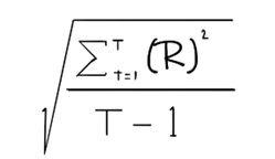
Where:
\((R)\) = Active return.
\(T\) = Total number of periods.
\(t\) = Active return at time t.
Needs to be redone
Active risk, also known as tracking error, represents the standard deviation of active returns. Portfolios with substantial fluctuations in active returns will exhibit high active risk. Generally, it’s preferable to minimize high active risk unless it’s a deliberate choice to seek higher returns, which might naturally result in greater risk.
$$ \begin{array}{l|l|l} \textbf{Style} & \textbf{Description} & {\textbf{Active Share} \\ \textbf{and Risk}} \\ \hline \text{Pure index} & \text{No active investing} & \text{Zero} \\ \hline \text{Factor Neutral} & {\text{No active factor bets, firm-} \\ \text{specific risk is low}} & \text{Low} \\ \hline \text{Factor Diversified} & {\text{Balanced exposure, firm-} \\ \text{specific risk is low}} & {\text{Low active risk; higher} \\ \text{active share}} \\ \hline {\text{Concentrated Factor} \\ \text{Bets}} & {\text{Targeted factor bets,} \\ \text{idiosyncratic risk is high}} & \text{High} \\ \hline {\text{Concentrated Stock} \\ \text{Picker}} & {\text{Targeted individual stock} \\ \text{bets}} & \text{Highest} \end{array} $$
Portfolio construction can be conceptually simplified as an optimization challenge, which typically comprises two key elements: an objective function representing the desired goal and a set of constraints that define the permissible actions. Portfolio managers aim to attain favorable results while operating within these defined boundaries. The nature of the objective function and the specifics of the constraints can provide insights into an investment manager’s philosophy and approach.
The concept of risk-adjusted return involves optimizing portfolio construction, with the specific approach determined by how risk is measured. If predicted active risk is the chosen metric, the goal is to maximize the information ratio (the ratio of active return to active risk). Alternatively, if predicted portfolio volatility is the risk measure, the objective is to maximize the Sharpe ratio (the ratio of return in excess of the risk-free rate to portfolio volatility). Ideally, these objective functions should account for implementation costs.
Typical constraints in portfolio optimization include limitations on geographic, sector, industry, and single-security exposures. They may also set constraints on transaction costs, exposure to specific factors, or metrics such as market capitalization and price-to-book ratios. Constraints can be defined relative to the benchmark or independently.
Finding the right balance in setting constraints that align with the risk dimensions, preferred risk level, and desired portfolio structure can be a challenging task. Essentially, the portfolio manager’s goal is to blend these objectives and constraints to maximize the chosen objective function while adhering to the defined limitations.
While not all portfolio managers follow a formal, scientific approach, most at least conceptually optimize their portfolios by considering expected returns, their own risk assessments, and any constraints established by the portfolio construction process or clients. This technical framework provides a structured way to discuss the portfolio construction process, even though the degree of formality may vary among managers.
$$ \begin{array}{l|c|c} & \textbf{Absolute Framework} & \textbf{Relative Framework} \\ \hline \textbf{Objective Function:} & \textit{Maximize Sharpe} & \textit{Maximize Information} \\ & \textit{Ratio} & \textit{Ratio} \\ \hline \underline{\textbf{Constraint}} & & \\ \hline {\text{Individual security} \\ \text{weights (w)}} & w_i \le 2\% & \mid w_{ip}-w_{ib} \mid \le 2\% \\ \hline \text{Sectors weights (S)} & S_i \le 2\% & \mid S_{ip}-S_{ib} \mid \le 2\% \\ \hline \text{Portfolio volatility } (\delta) & \delta_p \lt 0.9\delta_b \\ \hline – \text{Active risk (TE)} & – & TE\le 5\% \\ \hline {\text{Weighted average} \\ \text{capitalization (Z)}} & Z\ge 20bn & Z\ge 20bn \end{array} $$
Note the following:
Alternative optimization methods define their goals using risk metrics like portfolio volatility, downside risk, maximum diversification, and drawdowns. These methods do not explicitly include an expected return element, yet they inherently introduce exposure to risk factors.
A clear objective function, which could be defined by a quantitative manager aiming to maximize their exposure to beneficial factors can be derived as follows:
$$ \text{MAX}\left[\sum_{i=1}^N \frac {1}{3} \text{Size}_i+ \frac {1}{3} \text{Value}_i+ \frac {1}{3} \text{Momentum}_i \right] $$
Where \(\text{Size}_i\), \(\text{Value}_i\), and \(\text{Momentum}_i\) are standardized proxy measures of Size, Value, and Momentum for security i.
Question
Given the following data, portfolio active share is closest to?
Example 3
$$ \begin{array}{c|c|c} \textbf{Stock} & \textbf{Portfolio (P)} & \textbf{Benchmark (B)} \\ \hline A & 0.00 & 0.25 \\ \hline B & 0.10 & 0.25 \\ \hline C & 0.30 & 0.25 \\ \hline D & 0.60 & 0.25 \\ \hline & & \bf{\text{Active Share} = ?} \end{array} $$
- -0.10.
- 0.40.
- 0.10.
Solution
The correct answer is B.
Example 3
$$ \begin{array}{c|c|c|c} \textbf{Stock} & \textbf{Portfolio (P)} & \textbf{Benchmark (B)} & \bf{\mid P – B \mid} \\ \hline A & 0.00 & 0.25 & -0.25 \\ \hline B & 0.10 & 0.25 & -0.15 \\ \hline C & 0.30 & 0.25 & 0.05 \\ \hline D & 0.60 & 0.25 & 0.35 \\ \hline & & \textbf{Active Share} & \bf{0.4} \end{array} $$
$$ \begin{align*} \text{Step one: } & \mid -0.25 + -0.15 + 0.05 + 0.35 \mid = 0.80 \\ \text{Step two: } & 0.8 \times \frac {1}{2} = 0.4 \end{align*} $$
Reading 26: Active Equity Investing: Portfolio Construction
Los 26 (c) Discuss approaches for constructing actively managed equity portfolios
Offered by AnalystPrep


Get Ahead on Your Study Prep This Cyber Monday! Save 35% on all CFA® and FRM® Unlimited Packages. Use code CYBERMONDAY at checkout. Offer ends Dec 1st.