


Types of Dividends
A dividend is a distribution of profits paid to shareholders. The payment of... Read More

A carry arbitrage model is a no-arbitrage approach where the underlying asset is either sold or bought and a forward position established. This model accounts for the cost to hold or carry the underlying instrument. The carry costs for an underlying physical asset such as gold would be the financing cost plus insurance and storage costs. The carry arbitrage model also adjusts for dividends, and interest received, collectively referred to as carry benefits.
To bring the carry arbitrage model closer to real market conditions, we must address specific additional factors. There are carry arbitrage models when there are no underlying cash flows and carry arbitrage with underlying cash flows.
Let us assume that an arbitrageur has entered a forward contract to sell an underlying for delivery at time T. To reduce their exposure to market risk, they can buy the underlying at time 0 with borrowed money and carry it to the forward expiration date T. The risks of this scenario are:
$$ {\begin{array}{l|l|l} \textbf{}&{\textbf{Time}\\ (\textbf{0})}&{\textbf{Time}\\ (\textbf{T)}}\\ \hline {\text{Borrowing funds to} \\ \text{purchase and carry} \\ \text{an underlying} \\ \text{instrument}} \\ \hline \text{Underlying} & – S_0 \text{(Purchase)} & +S_T\text{(Sale)} \\ \hline \text{Borrowed Funds} & +S_0\text{(Inflow)} & -FV(S_0)\text{(Repayment)} \\ \hline \text{Net Cash Flow} & +S_0 -S_0=0 & +S_0-FV(S_0) \\ \hline \textbf{Short Forward}& V_0=0&V_T=F_0-S_T \\ \hline {\textbf{Overall Position:} \\ \textbf{Long Position} \\ \textbf{+Short Position} \\ \textbf{+Borrowed Funds}} \\ \hline &+S_0 -S_0+V_0=0& +S_T-FV(S_0)+V_T=0 \\ \hline & & {+S_T-FV(S_0) \\ +(F_0-S_T) =0} \\ \hline & &+F_0-FV(S_0)=0\\ \hline \textbf{Net} & 0 & F_0=FV(S_0) \\ \end{array}}$$
Using borrowed funds, the underlying investment is purchased at S0. Further, note that the asset can be sold at time T for ST. Moreover, the borrowed funds will be repaid at time T at the cost of FV(S0). It is equally noteworthy that our underlying transaction will suffer a loss when ST is below FV(S0). A short forward position will be added to the long position to offset any profit or loss, with both positions having no initial cash flow. The overall portfolio should have a value of zero at time T to prevent arbitrage. Most importantly, remember that there is no arbitrage profit when the initial agreed forward price \(F_0=FV(S_0)\).
Given that carry arbitrage rests on the no-arbitrage assumptions, the arbitrageur borrows money to purchase the underlying and lends money to sell the underlying. The borrowing and lending are done at a risk-free interest rate, and the arbitrage does not take any price risk. When we assume continuous compounding (rc), then \(F_0=FV(S_0)\) = \(S_0 e^{r_cT} \) and when we assume annual compounding (r), \(F_0=FV(S_0)\) = \(S_0 (1+r)^T \).
Let us use an example to illustrate the price exposure for holding the underlying investment.
Assume that company Z has a long financial position from carrying a non-dividend-paying stock. Further, assume that \(S_0\) = 100, r = 6% and T = 1. We allow the stock price to go up to \(S_T+\) = 110 and to decrease to \(S_T-\) = 90 at expiration. At the expiration date, the loan will be 100(1.06) = 106. At times, 0 and T, the initial transactions, will generate cash flows. The two transactions that produce a levered equity purchase at time 0 are:
At time T, the stock price will be \(S_T+\) =110 or \(S_T-\) = 90, which carries a price risk. After the loan repayment, if the stock price increases, the net cash flow will be 110 – 106 = +4 or – 16 if it decreases (90 – 106). We need to eliminate the price risk. To do this, we must add another step which is: Sell a forward contract to set price at F0 = 106 for the future sale of our underlying stock.
Since we have two outcomes, 110 or 90, at expiration, we short the forward. Consequently, there will be zero net cash flow at time T.
When stock price increases at time T:
\(S_T+=110\)
\(\text{Short Forward} (V_T) = F_0 – S_T =106-110 =- 4\)
\(CF_T^+ =S_T^+ -\text{Loan} +\text{Forward} = 110-106+(-4)=0\)
When stock price decreases at time T:
\(S_T- = 90\)
\(\text{Short Forward} (V_T) = F_0 – S_T = 106-90 = 14\)
\(CF_T^{-} =S_T^{+} -\text{Loan} + \text{Forward} = 90-106+14 = 0\)
Since there was no uncertainty about value at time T:
\(F_0\) = Future value of underlying stock = \(FV(S_0)\).
If \(F_0>FV(S_0)\), the forward contract will be sold, and the underlying stock bought. This has the effect of reducing the forward price and increasing the underlying price until \(F_0=FV(S_0)\). The risk-free positive cash flows will cease to exist. If \(F_0<FV(S_0)\), we buy the forward contract and sell the underlying short (reverse carry arbitrage) to increase the forward price and reduce the underlying price.
The quoted forward price does not directly reflect expectations of future underlying prices. The current price, the absence of arbitrage, time to expiration, and the interest rate are important. When we carry the asset, an assumption that the underlying price will increase in value does not affect the forward price. Once a forward contract has been entered, its fair value is derived from knowing if it will make or lose money.
To explain forward valuation, we will use the illustration below.
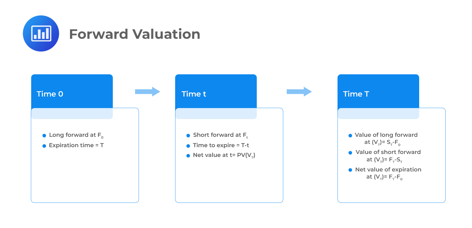 The first transaction will be the purchase of a forward contract at a price of \(F_0\) at time 0. Imagine selling a new forward contract at time \(t\) at a price of \(F_t\). Time \(t\), in this context, is the date of valuation of the forward contract. The offsetting forward entered at time \(t\) is not subject to market risk because the spot price does not affect the cash flow at time \(T\). The value of the original forward contract at the time entered at time 0 is \(PV(F_t-F_0)\) at time \(t\). Under annual compounding, the long forward value at time \(t\) is \(V_t\text{(long)}\) = Present value of the difference in forward prices:
Equation 1 below can be used when market frictions cause the forward price to differ from the correct arbitrage-free price.
$$ V_t= [F_t-F_0]= \frac {\left[F_t– F_0\right]}{(1+r)^{T-t}} $$
Where:
\(F_t\) = Current forward price.
\(F_0\) = Initial forward price.
Equation 2 below is used when the spot rate \(S_t\) is more readily observed than the forward price.
$$ V_t= S_t-[F_0]= S_t- \frac {F_0}{(1+r)^{T-t}} $$
The short forward contract value is the present value of the difference between the negative long position value and forward prices. Value of the short forward contract before maturity (Time \(t\)) = \(-V_t\).
$$ -V_t= [F_t-F_0]= \frac {\left[F_t– F_0\right]}{(1+r)^{T-t}} $$
or
$$ -V_t= S_t-[F_0]= \frac {F_0}{(1+r)^{T-t}} -S_t$$
Carry arbitrage requires payment of interest costs for borrowing funds to buy the underlying stock. Reverse carry arbitrage, on the other hand, requires receipt of interest benefit from lending the proceeds short-selling the underlying stock. There are other carry benefits and costs for many instruments which will be incorporated in forward pricing.
Carry benefits (CB) are the cash flows an investor might receive for holding the underlying instrument.
\(CB_T\) = The future value of underlying stock carry benefits at time \(T\).
\(CB_0)\) = The present value of underlying stock carry benefit at time 0.
Carry costs (CC) for commodities include storage, insurance, and waste management expenses. Carry cost for financial instruments are 0.
\(CC_T\) = The future value of underlying carry cost at time \(T\).
\(CC_0\) = The present value of underlying carry cost at time 0.
Holding financial assets results in the opportunity cost of the interest earned on the money tied to carrying the spot asset; thus, they have no direct carry cost. To determine a forward price, the cost to finance the spot asset purchase, storage cost, and any benefit from holding the asset, will all be used. The forward pricing equation is expressed as:
\(F_0\) = Future value of the underlying adjusted for cash flows =\(FV[S_0+CC_0-CB_0]\)
The equation above is called the future-spot parity of cost of carry model and considers the carry cost in relation to the forward price of an asset to the spot price. These costs are added to the equation because the carry costs and a positive interest rate increase the burden of carrying the underlying asset over time. On the other hand, carry benefits reduce the burden of carrying the underlying asset over time; thus, the benefits are deducted from the equation.
Many financial assets do not have carry cost; hence the equation for such assets will be:
$$F_0=FV(S_0)-CB_0=FV(S_0)-\text{Benefit}$$
For a dividend-paying stock, the benefit will be the dividend (D). The future value computation for the dividends will differ from that of the stock price because the future value is only compounded from the time the dividend is received to the day when the forward expires. Hence for a dividend received at time t and held until time \(T\), the equation would be,
$$FV[PV(D)]=FV[\frac{D}{(1+r)^t} ]=(1+r)^t ×[(\frac{D}{(1+r)^t })]=D(1+r)^ {T-t}$$
The long forward position when the underlying with carry costs and benefits is calculated the same way as in the previous discussion, but the initial forward price and the new forward price are adjusted for the benefits and costs.
\(V_t\) is the present value of the difference in forward prices adjusted for carry benefits and costs:
$$ V_t = PV[F_t-F_0] $$
Where:
\(F_t\)=\(FV(S_t+CC_t-CB_t)\)
\(F_0\)=\(FV(S_0+CC_0-CB_0)\)
A UK stock that pays a £20 dividend in two months is trading at £2000. The UK interest rate is 6% with annual compounding. Based on the no-arbitrage approach and the current stock price, the equilibrium three-month forward price will be closest to:
$$ F_0 =FV(S_0)-(D) $$
\(S_0\) = £2000, \(r\) = 6% and \(T\) = 3/12
$$ \begin{align} F_0 & =2,000(1+0.06)^{3⁄12}-20(1+0.06)^{1⁄12} \\ & =£2,029.35 – £20.097 \\ & = £2,009.253 \end{align}$$
When dealing with index stock, it isn’t easy to account for the many dividend payouts by the underlying stock with varying amounts and time. The dividend index point solves this problem by measuring the number of dividends attributable to a particular index. A continuous dividend yield is assumed to simplify the problem. This means that we assume that the dividends continuously accrue throughout the contract rather than having dividends paid on specific dates. The carry costs and benefits can be expressed as:
$$ F_0=S_0e^{(r_c+CC-CB)T} $$
Where rc, CC, and CB are continuously compounding rates.
Question
Assume that at time 0, a one-year forward contract was entered with a price of 106. Six months later, at time t= 0.5, the underlying asset’s price is S0.5 = 112, and the interest rate is 6%. The value of the existing forward in six months is likely to be:
- 9.
- 9.3.
- 9.043.
Solution
The correct answer is C.
\(T-t= 1 -0.5= 0.5\)
The six months forward price at time t is
$$F_t=FV(S_t )=112(1+0.06)^{0.5}=115.311$$
The value of the existing forward will be the difference between \(F_t\) and \(F_0\).
$$ V_t= [F_t-F_0]= \frac {\left[115.311– 106\right]}{(1+0.06)^{0.5}} = 9.043$$
Reading 33: Pricing and Valuation of Forward Commitments
LOS 33 (a) Describe the carry arbitrage model without underlying cash flows and with underlying cashflows.
Offered by AnalystPrep


Get Ahead on Your Study Prep This Cyber Monday! Save 35% on all CFA® and FRM® Unlimited Packages. Use code CYBERMONDAY at checkout. Offer ends Dec 1st.