


Study Notes for CFA® Level II – Eth ...
Reading 45: Code of Ethics and Standards of Professional Conduct -a. Describe the... Read More

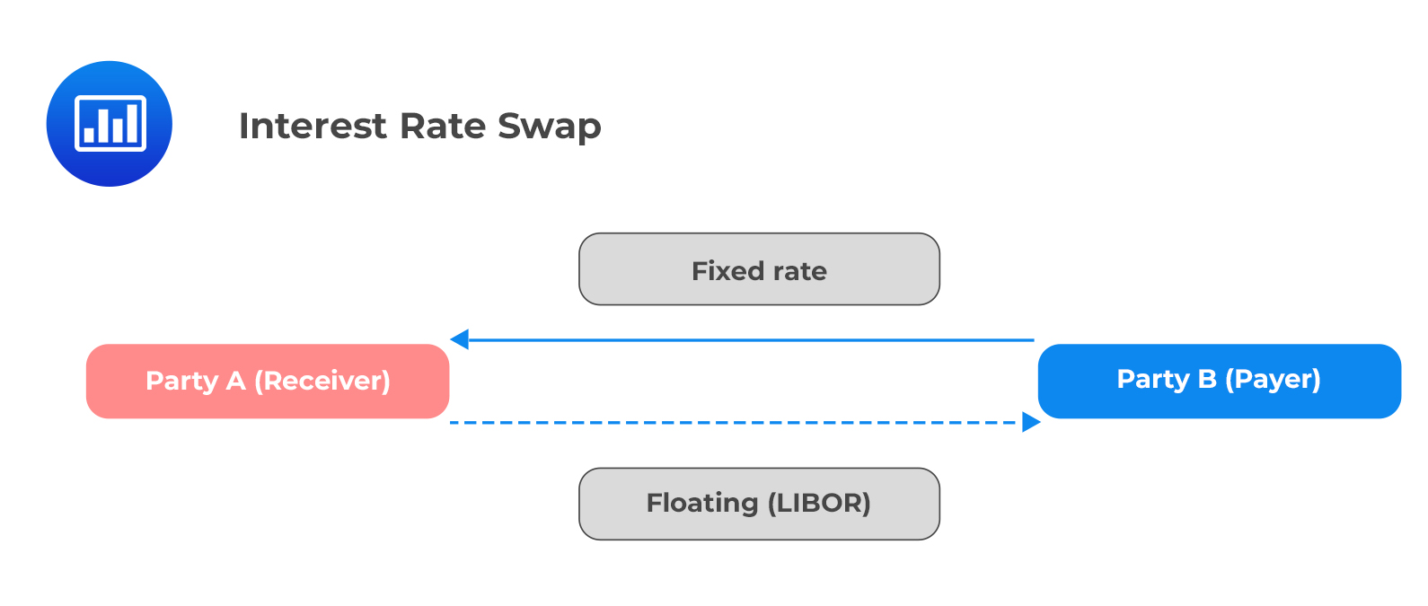
An interest rate swap is a contract to exchange interest rate payments in the future between two parties over a specified period.
Vanilla interest rate swaps (most commonly traded and most liquid) are contracts to exchange a fixed interest rate for a floating rate. The converse is also true. Each party is associated with a fixed leg and a floating leg.
 The swap rate is the fixed interest rate demanded by the receiver of a swap to exchange the uncertain floating rate payments over time. The forward curve shows the market’s forecast of future floating interest rates.
The swap rate curve or swap curve is a par curve showing swap rates over all the available maturities.
Swap contracts are non-standardized customizable contracts between two parties in the over-the-counter market. This implies that they bear counterparty risk. The value of a swap at the contract initiation is zero.
The swap curve is a powerful indicator of conditions in the fixed income markets as it shows both floating rate expectations and bank credit.
The choice between government bond spot curves and swap curves as a benchmark for the time value of money in fixed income valuation depends on the relative liquidity of the concerned markets.
Wholesale banks use the swap curve to value assets and liabilities because they hedge many items on their balance sheets with swaps.
On the other hand, retail banks have low exposure to the swap market. Therefore, they are more likely to use the government spot curve as their benchmark.
When pricing a swap, we need to determine the present value of the fixed and floating legs. It is straightforward to calculate the fixed leg as the future cash flows are set at the beginning of the contract. On the contrary, the floating leg is based on future interest rates, which vary with time, making it complex to calculate.
The swap rate can be determined using the following formula:
$$ \begin{align*} \sum_{t=1}^{T}&{\frac{\text{Swap Rate at time T}}{\left(1+S\left(t\right)\right)^t}+\frac{1}{\left(1+S\left(T\right)\right)^T}} \\ & = 1 (\text{Value of the floating leg at swap initiation}) \end{align*} $$
Where:
\(S(t)\) and \(S(T)\) are spot rates at time \(t\) and \(T\) respectively.
This formula is based on the concept that the total value of the swap’s fixed payments is equal to the expected floating payments’ value implied by the forward floating curve at the beginning of the swap agreement.
Consider the following spot curve for different maturities.
$$ \begin{array}{c|c} \textbf{Year} & \textbf{Spot Rate} \\ \hline 1 & 2.00\% \\ \hline 2 & 4.00\% \\ \hline 3 & 6.00\% \\ \hline 4 & 7.00\% \end{array} $$
Use the information in the above table to determine the swap rate curve.
Solution
$$ \sum_{t=1}^{T}{\frac{\text{Swap Rate at time}(SR_T)}{\left(1+S\left(t\right)\right)^t}+\frac{1}{\left(1+S\left(T\right)\right)^T}=1} $$
For T=1,
$$ \begin{align*} \frac{SR_1}{1.02}+\frac{1}{1.02} &=1 \\ SR_1 &=2\% \end{align*} $$
For T=2,
$$ \begin{align*} \frac{SR_2}{1.02}+\frac{SR_2}{\left(1.04\right)^2}+\frac{1}{{1.04}^2}& =1 \\ SR_2 &=3.96\% \end{align*} $$
For T=3,
$$ \begin{align*} \frac{SR_3}{1.02}+\frac{SR_3}{{1.04}^2}+\frac{SR_3}{{1.06}^3}+\frac{1}{{1.06}^3}&=1 \\ SR_3 &=5.84\% \end{align*} $$
Question
A government spot curve implies the following discount factors. The swap rates for years 1, 2, and 3 are closest to:
$$ \begin{array}{c|c} \textbf{Year} & \textbf{Discount Factor} \\ \hline 1 & 0.9963 \\ \hline 2 & 0.9916 \\ \hline 3 & 0.9854 \end{array} $$
- 0.37%; 0.42%; 0.49%.
- 0.37%; 0.85%; 1.48%.
- 0.37%; 1.70%; 4.51%.
Solution
The correct answer is A.
Firstly, we need to calculate the spot rates from the discount factors given.
$$ P\left(T\right)=\frac{1}{\left(1+S\left(T\right)\right)^T} $$
For T=1,
$$ \begin{align*} 0.9963 &=\frac{1}{1+S_1} \\ S_1 &=0.37\% \end{align*} $$
To determine the swap rate, use the formula:
$$ \sum_{t=1}^{T}{\frac{\text{Swap Rate at time}(SR_T)}{\left(1+S\left(t\right)\right)^t}+\frac{1}{\left(1+S\left(T\right)\right)^T}=1} $$
$$ \begin{align*} &=\frac{SR_1}{1.0037}+\frac{1}{1.0037} =1 \\ SR &=0.37\% \\ 0.9916 & =\frac{1}{\left(1+S_2\right)^2} \\ S_2 &=0.42\% \\ & =\frac{SR_2}{1.0037}+\frac{SR_2}{\left(1.0042\right)^2}+\frac{1}{\left(1.0042\right)^2} =1 \\ SR_2 &=0.42\% \\ 0.9854 & =\frac{1}{\left(1+S_3\right)^3} \\ S_3 &=0.49\% \\ &= \frac{SR_3}{1.0037}+\frac{SR_3}{\left(1.0042\right)^2}+\frac{SR_3}{\left(1.0049\right)^3}+\frac{1}{\left(1.0049\right)^3} =1 \\ SR_3 & =0.49\% \end{align*} $$
Thus, the swap rates are as given in the following table:
$$ \begin{array}{c|c|c|c} \textbf{Year} & \textbf{Discount Factor} & \textbf{Spot rate} & \textbf{Swap Rate} \\ \hline 1 & 0.9963 & 0.37\% & 0.37\% \\ \hline 2 & 0.9916 & 0.42\% & 0.42\% \\ \hline 3 & 0.9854 & 0.49\% & 0.49\% \end{array} $$
Reading 28: The Term Structure and Interest Rate Dynamics
LOS 28 (e) Explain the swap rate curve and why and how market participants use it in valuation.
Strengthen your CFA Level II fixed-income skills with exam-style practice on swap curves, bond valuation, and interest-rate term structure analysis.
Offered by AnalystPrep


Get Ahead on Your Study Prep This Cyber Monday! Save 35% on all CFA® and FRM® Unlimited Packages. Use code CYBERMONDAY at checkout. Offer ends Dec 1st.