Time-series Data vs. Cross-sectional Data

Time-series Data

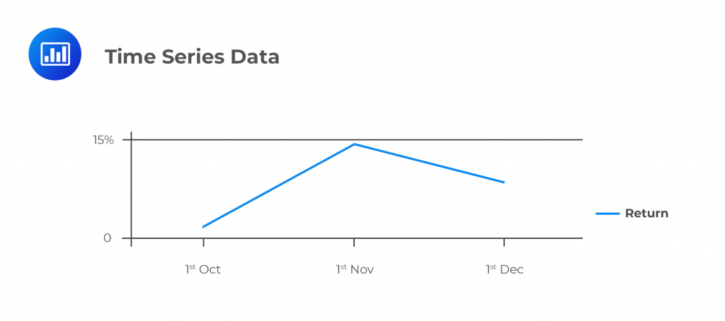
Time-series data refers to a set of observations made over a given period of time at specific and equally-spaced time intervals. That the observations are made at specific points in time means time intervals are discrete.

A good example of time-series data could be the daily or weekly closing price of a stock recorded over a period spanning 13 weeks. Other appropriate examples could be the set of monthly profits (both positive and negative) earned by Samsung between the 1^st of October 2018 and the 1^st of December 2018.

Time-series data can be used to predict the future values of a given financial vehicle. Although such past data may help estimate future values, it’s always important to note that the future and the past are independent. Therefore, past performance may not always be indicative of future performance.

Time-series data has at least one systematic pattern, with the most common patterns being either trends or seasonality. Since most trends are linear or quadratic, regression analysis and the moving average method establish the linear relationship between variables.

Seasonality, on the other hand, is a trend that systematically keeps on repeating itself over time. Numerous modern computer-based programs are used to analyze time-series data, including SPSS, JMP, SAS, Matlab, and R.

Cross-sectional Data

Cross-sectional data refers to a set of observations made at a single point in time. Samples are constructed by collecting the data of interest across a range of observational units – people, objects, firms – simultaneously.

A good example of cross-sectional data can be the stock returns earned by shareholders of Microsoft, IBM, and Samsung for the year ended 31^st December 2018.

It is possible to pool time series data and cross-sectional data. If we were to study a particular characteristic or phenomenon across several entities over a period of time, we would end up with what is referred to as panel data. For example, suppose we study the GDP of 3 developing countries for a period spanning 3 years, say, from 2015 to 2017:

$$ \begin{array}{c|c|c} \text{Country} & \text{Year} & \text{GDP} \\ \hline \text{Kenya} & {2015} & {–} \\ \text{Kenya} & {2016} & {–} \\ \text{Kenya} & {2017} & {–} \\ \text{India} & {2015} & {–} \\ \text{India} & {2016} & {–} \\ \text{India} & {2017} & {–} \\ \text{Brazil} & {2015} & {–} \\ \text{Brazil} & {2016} & {–} \\ \text{Brazil} & {2017} & {–} \\ \end{array} $$

Here, we would study a group of entities (Kenya, India, and Brazil) over a period of time (3 years). This would constitute panel data.