Measures of Central Tendency

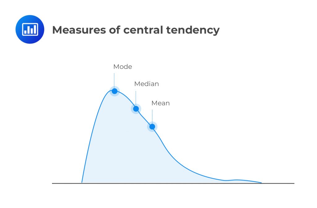
Measures of central tendency are values that tend to occur at the center of a well-ordered data set. As such, some analysts call them measures of central location. Mean, median, and mode are all measures of central tendency. Even then, there are situations in which, compared to the others, one is the most appropriate. The mean is the most common among the three measures. It can also be subdivided into smaller sub-types, as we shall see shortly.

Population vs. Sample

A population includes all of the elements from a set of data. A sample, on the other hand, consists of a few observations drawn from the population. For example, all domestic equity mutual funds available in a country’s market qualify to be called a population. If 15 domestic equity mutual funds are selected from among all the domestic equity mutual funds, then this is a sample.

Uses of Sample

• Since collecting data from every element in a population is very difficult, samples can be used to represent the population.
• The use of a sample saves time and makes the analysis of a large population manageable.

A parameter refers to a measure that is used to describe a characteristic of the population. It’s a numerical quantity that describes a given aspect of the population as a whole.

A statistic, on the contrary, is a measure that describes a characteristic of a sample. This could be the average value or the sample standard deviation of the sampled items. Researchers use sample statistics to estimate the unknown population parameters. For example, we often estimate the actual population mean using the sample mean.

Arithmetic Mean

The population mean is the summation of all the observed values in a population, \(\sum{X_i}\) divided by the total number of observations, \(N\). The population mean differs from the sample mean, which is based on a few observed values ‘\(n\)’ that are chosen from the population. Thus:

$$\begin{align} \text{Population mean} &=\cfrac { \sum { { X }_{ i } } }{ N }\\ \text{Sample mean} &=\cfrac { \sum { { X }_{ i } } }{ n } \end{align}$$

Analysts use the sample mean to estimate the actual population mean.

• The population mean and the sample mean are both arithmetic means. The arithmetic mean for any data set is unique and is computed using all the data values. Among all the measures of central tendency, it is the only measure for which the sum of the deviations from the mean is zero.

Example: Calculating the Arithmetic Mean

The following are the annual returns realized from a given asset between 2005 and 2015.

{ 12%   13%   11.5%   14%   9.8%   17%   16.1%   13%   11%   14% }

1. Calculate the population mean.

2. Compute the sample mean assuming the returns for the first 7 years are unknown, i.e., we only have 13%, 11%, and 14%.

Solution

$$ \begin{align*} \text{Population mean} & =\cfrac {(0.12 + 0.13 + 0.115 + 0.14 + 0.098 + 0.17 + 0.161 + 0.13 + 0.11 + 0.14)}{10} \\ & = 0.1314 \text{ or } 13.14\% \\ \\ \text {Sample mean} & = \cfrac {(0.13 + 0.11 + 0.14)}{3} \\ & = 0.1267 \text{ or } 12.67\% \\ \end{align*} $$

A commonly-cited demerit of the arithmetic mean is that it’s not resistant to the effects of extreme observations or what we call ‘outsider values.’ For instance, consider the following data set:

{1   3   4   5   34}

The arithmetic mean is 9.4, which is greater than most of the values. This is due to the last extreme observation, i.e., 34.

Properties of the Arithmetic Mean 

• The sum of the deviations around the mean always equals 0.
• The arithmetic mean is highly sensitive to extremely large or small observations (outliers).

Trimmed Mean

The trimmed mean is a measure of central tendency in which we calculate the mean by excluding a small percentage of the lowest and highest values. For example, we calculate the mean in a 5% trimmed mean by removing the lowest 2.5% and the highest 2.5% of values.

Winsorized mean

The Winsorized mean is a measure of central tendency. It is calculated by assigning a stated percentage of the lowest values equal to one specified low value and a stated percentage of the highest values equal to one specified high value. In the same way, as the trimmed mean, this approach removes a significant number of outliers from a data set.

Weighted Mean

The weighted mean takes the weight of every observation into account. It recognizes that different observations may have disproportionate effects on the arithmetic mean. Thus:

$$ \text{Weighted mean} = \sum { { X }_{ i }{ W }_{ i } } $$

Example: Calculating the Weighted Mean

A portfolio consists of 30% ordinary shares, 25% T-bills, and 45% preference shares with returns of 7%, 4%, and 6%, respectively. The portfolio return is closest to:

Solution

The return of any portfolio is always the weighted average of the returns of individual assets. Thus:

$$ \text{Portfolio return} = (0.07 × 0.3) + (0.04 × 0.25) + (0.06 × 0.45) = 5.8\% $$

Geometric Mean

The geometric mean is a measure of central tendency, mainly used to measure growth rates. We define it as the n^th root of the product of n observations:

$$ \text{GM} ={ \left( { X }_{ 1 }\ast { X }_{ 2 }\ast { X }_{ 3 }\ast { X }_{ 4 }\ast …\ast { X }_{ n-1 }\ast { X }_{ n } \right) }^{ \frac { 1 }{ n } } $$

The formula above only works when we have non-negative values. To solve this problem, especially when dealing with percentage returns, we add 1 to every value and then subtract 1 from the final result.

Example: Calculating the Geometric Mean

An ordinary share from a certain company registered the following rates of return over a 6-year period:

{ -4%   2%   8%   12%   14%   15% }

The compound annual rate of return for the period is closest to:

Solution

$$ \text{Geometric Mean} = (0.96 × 1.02 ×1.08 × 1.12 × 1.14 × 1.15)^{\frac{1}{6}} = 1.0761 – 1 = 0.0761 \text{ or } 7.61 % $$

Computing Geometric Mean Using BA II Plus™ Financial Calculator:

Enter 1.55280 [y^x] 6 [1/x] [=]

Where 1.55280 = 0.96 × 1.02 ×1.08 × 1.12 × 1.14 × 1.15

Important Points Related to the Geometric Mean and the Arithmetic Mean

• The geometric mean is always less than or equal to the arithmetic mean.
• The geometric mean is equal to the arithmetic mean when there is no variability in the observations (when all the observations in the series are the same).
• The gap between the geometric mean and the arithmetic widens as the variability of values increases.
• The arithmetic mean should be used for estimating the average return over a one-period horizon.
• For estimating the average returns over more than one period, the geometric mean should be used.

Relationship between Arithmetic Mean and Geometric Mean

The relationship between the arithmetic mean and geometric mean is given by:

$$\bar{X}_G \approx \bar{X}-\frac{s^2}{2}$$

Where:

\(\bar{X}_G\) = Geometric mean.

\(\bar{X}\) = Arithmetic mean.

\(s^2\) = Sample variance.

The above equation shows that the larger the variance of the sample, the wider the difference between the geometric mean and the arithmetic mean.

Harmonic Mean

Analysts use the harmonic mean to determine the average growth rates of economies or assets. If we have \(N\) observations:

$$ \text{HM} = \cfrac {N}{ \left(\sum { \frac { 1 }{ { X }_{ i } } } \right)} $$

Example: Calculating the Harmonic Mean

For the last three months of 2015, the price of a stock was $4, $5, and $7, respectively. The average cost per share is closest to:

Solution

$$\text{Harmonic Mean}=\frac{3}{\left(\frac{1}{4}+\frac{1}{5}+\frac{1}{7}\right)}=\$ 5.06$$

Important Points Related to the Harmonic Mean

• \(\text{Harmonic mean < Geometric mean < Arithmetic mean when returns are variable.}\)
• \(\text{Harmonic mean = Geometric mean = Arithmetic mean when returns are constant.}\)
• \(\text{Arithmetic mean × Harmonic mean = Geometric mean.}\)

Median

The median is the statistical value located at the center of a data set organized in the order of magnitude. For an odd number of observations, the median is simply the middle value. If the number of observations is even, the median is the middle point (average) of the two middle values. Unlike the arithmetic mean, the median is resistant to the effects of extreme observations.

Example: Calculating the Median

The following are the annual returns on a given asset realized between 2005 and 2015.

{ 12%   13%   11.5%   14%   9.8%   17%   16.1%   13%   11%   14% }

The median is closest to:

Solution

First, we arrange the returns in ascending order:

{ 9.8%   11%   11.5%   12%   13%   13%   14%   14%   16.1%   17% }

Since the number of observations is even, the median return will be the middle point of the two middle values:

$$\frac{13\%+13\%}{2}=13\%$$

The main advantage of the median is that the median is less affected by outliers than the mean. Therefore, the median is useful in describing data that follow a non-symmetric distribution, such as a skewed distribution, which we will see later in this reading.

Limitations of the Median

• The median only focuses on the relative position of the ranked observation and ignores the rest of the information about the size of the obser­vations.

Mode

The mode is the value that occurs most frequently in a data set. On a histogram, it is the highest bar. A data set may have a mode or none, e.g., the returns in the example above. One of its major merits is that it can be determined from incomplete data, provided we know the observations with the highest frequency.

If a distribution has two modes, it is called bimodal. If the distribution has the three most frequently occurring values, then it is called trimodal.

An interval with the highest frequency is called the modal interval (or intervals) in a frequency distribution. In a histogram, the modal interval always has the highest bar. The mode is the only measure of central tendency that can be used with nominal data.

Example: Calculating the Mode

Determine the mode from the following data set:

{ 20%   23%   20%   16%   21%   20%   16%   23%   25%   27%   20% }

Solution

The mode is 20%. It occurs 4 times, a frequency higher than that of any other value in the data set.