Calculation and Interpretation of Confidence Intervals

Confidence interval (CI) refers to a range of values within which statisticians believe the actual value of a certain population parameter lies. It differs from a point estimate which is a single, specific numerical value.

Breaking Down Confidence Interval

When constructing confidence intervals, we must specify the probability that the interval contains the true value of the parameter of interest. This probability is represented by (1 – α), where α is the level of significance. In statistical terminology, 1- α is called the degree of confidence or certainty.

We define a 100(1 – α)% confidence interval for a given parameter, say θ, by specifying two random variables, θ’₁(X) and θ’₂(X), such that P{θ’₁(X?) < θ < θ’₂(X)} = 1 – α.

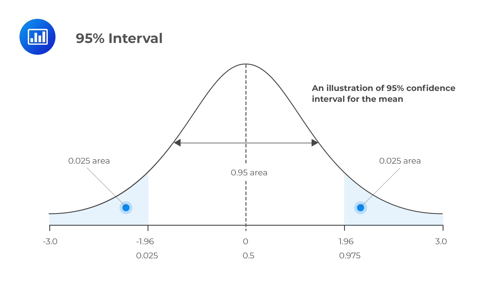
It happens that α = 0.05 is the most common case in examinations and practice. This leads to a 95% confidence interval.

Consequently, P{θ’₁(X) < θ < θ’₂(X)} = 0.95 specifies {θ’₁(X), θ’₂(X)} as a 95% confidence interval for θ. The main task for candidates lies in their ability to construct and interpret a confidence interval. Therefore, the CI for θ above could be interpreted to mean that if we were to construct similar intervals using samples of equal sizes from the same population, then 95% of the intervals would contain the true parameter value. Only 5% would not contain the true parameter value, hence, the phrase “confidence” interval.

Constructing Confidence Intervals

To construct a confidence interval, one must come up with an appropriate value that will be subtracted and added to a point estimate. A confidence interval appears as follows:

$$ \text C.\text{I} =\text{point estimate} \pm \text{reliability factor} * \text{standard error} $$

Where:

Point estimate refers to a calculated value of the sample statistic such as the mean, X.

The reliability factor is a value that depends on the sampling distribution involved and (1 – α), the probability that the point estimate is contained in the confidence interval.

$$ \text{Standard error} =\text {Standard error of the point estimate} $$

Different Scenarios

1. Normal Distribution With a Known Variance

We can calculate the confidence interval for the mean as,

$$ x \pm z_{\alpha/2} * \frac {\sigma}{\sqrt n} $$

Here, the reliability factor is z_α/2. The z-score leaves a probability of α/2 on the upper tail (right-hand tail) of the standard normal distribution.

The following table represents the standard normal distributions commonly used by analysts.

$$ \begin{array}{c|c|c} \text{Degree of confidence} & \text{Level of significance(one-tailed)} & {z_{\alpha/2}} \\ \hline {90\%} & {10\%} & {1.645} \\ \hline {95\%} & {5\%} & {1.960} \\ \hline {99\%} & {1\%} & {2.575} \\ \end{array} $$

2. Normal Distribution With Unknown Variance

When the variance is unknown, we construct the confidence interval for the mean by replacing the z-score in the first scenario with the t-score. Similarly, we replace the unknown σ with S, the standard deviation of the sample mean. Thus,

$$ CI = x \pm t_{\alpha/2} * \frac {S}{\sqrt n} $$

t_α/2 is the t-score that leaves a probability of α/2 on the upper tail of the t-distribution. The number of degrees of freedom is determined by the sample size such that the degrees of freedom (df) = n – 1.

3. The Confidence Interval of the Population Mean When Variance is Unknown, and the Sample Size is Large Enough (Any Distribution)

Thanks to the Central Limit Theorem, we can approximate just about any abnormal distribution as a normal one, provided the sample size is large (n ≥ 30). Therefore, we can use the relevant z-score when constructing a confidence interval for the population mean.

However, some analysts may advocate using the t-distribution in scenarios where the distribution is abnormal, and the population variance is unknown, even if n ≥ 30. Nonetheless, the use of the z statistic would still be justified under such circumstances, provided the Central Limit Theorem is applied correctly.

Example: Confidence Interval

A teacher draws a sample of five 12-year-old children from a school’s population and records their heights in centimeters as follows:

$$ \{124, 124, 128, 130, 127\} $$

Assume that the heights have a normal distribution where both μ and σ are unknown. Calculate a two-tailed 95% confidence interval for the mean height of the 12-year-old children.

Solution

Since the variance is unknown and the sample size is less than 30, we should use the t-score instead of the z-score, even if the distribution is normal. Therefore, the confidence interval for the mean will take the form illustrated below.

$$ CI = x \pm t_{\alpha/2} * \frac {S}{\sqrt n} $$

From the data, X = 126.6 and S² = 6.8

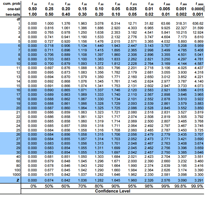
You can read off the t-score value from the t-distribution table where you will find that,

$$ t_{4, 0.025} = 2.776 $$

Please refer to the t-table below to find the critical t-value.

Therefore,

$$ \begin{align*}
CI & = 126.6 \pm 2.776 \times \frac {\sqrt 6.8}{\sqrt 5} \\
& = 126.6 \pm 3.2373 \\
\end{align*} $$

In view of the foregoing, our confidence interval for μ is (123.36, 129.84)

Question

Use data from the example above to calculate a two-tailed 99% confidence interval for the population mean.

A. (125.3, 127.91)

B. (117.9, 135.3)

C. (116.6, 136.6)

Solution

The correct answer is A.

$$ CI = x \pm t_{\alpha/2} * \frac {S}{\sqrt n} $$

$$ t_{4, 0.005 }= 4.604 $$

The other inputs remain the same as in the example above.

Therefore,

$$ \begin{align*}
CI & = 126.6 \pm 4.604* \frac {\sqrt 6.8}{\sqrt 5} \\
& = 126.6 \pm 5.4391 \\
\end{align*} $$

The confidence interval for the mean is (121.16, 132.01).

As you might have observed, the interval widens as the level of confidence increases.

Reading 10 LOS 10j:

Calculate and interpret a confidence interval for a population mean, given a normal distribution with 1) a known population variance, 2) an unknown population variance, or 3) an unknown variance and a large sample size.