Chi-square Test of a Single Population Variance and F-test of the Ratio of Two Population Variances

Testing the Variances of a Normally Distributed Population using the Chi-square Test

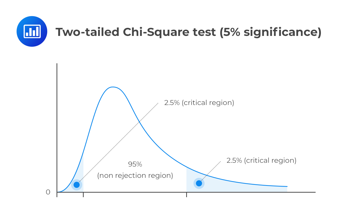
A chi-square test is used to establish whether a hypothesized value of variance is equal to, less than, or greater than the true population variance. Unlike most distributions covered in the CFA® Program curriculum, the chi-square distribution is asymmetrical. However, the distribution approaches the “normal” one as the degrees of freedom increase.

As a natural consequence, the chi-square distribution has no negative values and is bounded by zero. A chi-square statistic with (n – 1) degrees of freedom is computed as:

$$ { \chi }_{ n-1 }^{ 2 }=\frac { \left( n-1 \right) { S }^{ 2 } }{ { \sigma }_{ 0 }^{ 2 } } $$

Where:

\(n\) = Sample size.

\(S^2\) = Sample variance.

\({ \sigma }_{ 0 }^{ 2 }\) = Hypothesized population variance.

Example: Chi-square Test

For the 15-year period between 1995 and 2010, ABC’s monthly return had a standard deviation of 5%. John Matthew, CFA, wishes to establish whether the standard deviation witnessed during that period still adequately describes the long-term standard deviation of the company’s return. To achieve this end, he collects data on the monthly returns recorded between 1^st January, 2015 and 31^st December, 2016 and computes a monthly standard deviation of 4%.

Carry out a 5% test to determine if the standard deviation computed in the latter period is different from the 15-year value.

Solution

As is the norm, start by writing down the hypothesis

\(H_0: \sigma_0^2= 0.0025\)

\(H_1: \sigma^2 \neq 0.0025\)

Since the latter period has 24 months, n = 24. The test statistic is:

$$ { \chi }_{ 24-1 }^{ 2 }=\frac { \left( 24-1 \right) { 0.0016 } }{ 0.0025 } =14.72 $$

This is a two-tailed test. As such, we have to divide the significance level by two and screen our test statistic against the lower and upper 2.5% points of \({ \chi }_{ 23 }^{ 2 }\).

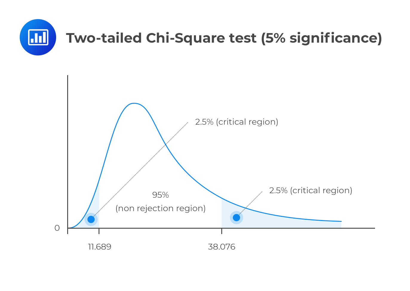
Consulting the chi-square table, the test statistic (14.72) lies between the lower (11.689) and the upper (38.076) 2.5% points of the chi-square distribution.

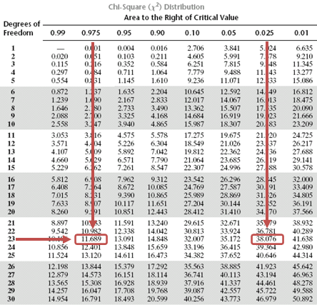
Therefore, we have insufficient evidence to reject the H₀. It is, therefore, reasonable to conclude that the latter standard deviation value is close enough to the 15-year value.

Testing the Equality of the Variances of Two Normally Distributed Populations based on Two Independent Random Samples using the F-distribution

Assume that we have 2 independent random samples of sizes n₁ and n₂ from \(N(\mu_1, \sigma_1^2)\) and \(N(\mu_2, \sigma_2^2)\).

Also, let us consider a scenario where we have the sample variances as \(S_1^2\) and \(S_2^2\). The basic situation usually involves the following hypothesis:

\(H_0: \ \sigma_1^2 =\sigma_2^2\)

\(H_1: \ \sigma_1^2 \neq \sigma_2^2\)

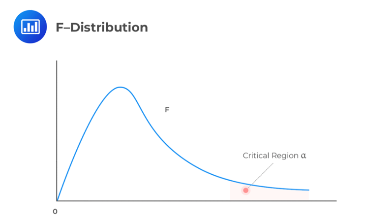
The test statistic is \(\frac {S_1^2}{S_2^2} \sim F_{n1 – 1, n2 – 1 } \text{ under } H_0\).

The decision rule is to reject the null hypothesis if the test statistic falls within the critical region of the F-distribution.

Example: F-test

Use the following data to calculate the test statistic. Establish if the variances of the two populations “A” and “B” can be considered to be equal at the 95% confidence level.

\(\sum A^2 =  56,430\) and \(\sum B^2 = 59,520\) and \(\bar{A}= 75\) while \(\bar{B} = 77\), \(n_1 = 10\) and \(n_2 = 10\)

Solution

First, state the hypothesis

\(H_0: \ \sigma_A^2 = \sigma_B^2\)

\(H_1: \ \sigma_A^2 \neq \sigma_B^2\)

Using the formula:

$$Var(X)=s^2=\frac{1}{n-1}\left[\sum{X^2}-n\bar{X}^2\right]$$

We have:

$$ \begin{align*} S_A^2 & =\cfrac { \left\{ 56,430 – (10 × 75^2) \right\} }{9} = 20 \\ S_B^2 & =\cfrac { \left\{ 59,520 – (10 × 77^2) \right\} }{9} = 25.556 \\ \end{align*} $$

Now,

$$ \cfrac {S_A^2}{ S_B^2}=\cfrac {20}{25.556} = 0.783 $$

We should compare the test statistic with the upper and lower 2.5% points of the F-distribution. These points are 4.026 and 1/4.026 = 0.2484. Since the test statistic lies between the two limits, we have insufficient evidence against the H₀. Therefore, it would be reasonable to conclude that the two samples have equal variance.