Bond Price Calculation

The price of a bond is influenced by various factors, including its cash flow features and market discount rate. The cash flow features are periodic payments made to bondholders, such as interest or coupon payments. On the other hand, the market discount rate is the required return based on the bond’s risk. It reflects investors’ expectations and the time value of money. At issuance, the bond price equals the present value (PV) of future interest and principal cash flows.

The price of a bond can be determined using mathematical formulas or spreadsheet functions as highlighted below:
Bond price: \( P=\sum_{t=1}^N \left( \frac{C_t}{(1+r)^t} \right) + \frac{FV_N}{(1+r)^N} \)

Where:

• r = Market discount rate.
• C_t = Coupon payment at time t.
• N = Number of periods until maturity.
• FV = Face value of the bond.
• PV of Bond coupon = \( \left( \frac{C_t}{\left(1+r\right)^t} \right) \).

Spreadsheet Function for Bond Price: Bond Price=PV (rate, nper, pmt, FV, type)
Where:

• Rate is the market discount rate per period.
• nper is the number of periods.
• pmt is the coupon payment per period.
• FV is the face value.
• Type refers to whether payments are made at each period’s end (0) or beginning (1).

Types of Bonds

Bonds are categorized into three main types, each representing a specific relationship between price, coupon rate, and market discount rate:

• Par bond: Price equals future value; coupon rate equals the market discount rate.
• Discount bond: Price is less than future value; coupon rate is less than the market discount rate.
• Premium bond: Price is greater than future value; coupon rate is greater than the market discount rate.

Yield-to-Maturity (YTM)

Yield-to-maturity (YTM) represents the bond’s internal rate of return (IRR), which is the single, uniform interest rate that, when applied to discount the bond’s future cash flows, equals the bond’s current price. In essence, YTM is the implied or observed market discount rate. It is also known as the bond’s “promised yield,” assuming the issuer does not default. YTM (“yield”) is used interchangeably with market discount rate or required yield. Instead of discussing bond prices, market participants might say “yields are rising” to mean “market discount rates are rising” or “bond prices are falling.”

Conditions for Earning YTM

An investor will achieve a return equal to the YTM if the following conditions are met:

• Holding the bond until maturity.
• Receiving full coupon and principal payments on the scheduled dates from the issuer.
• Reinvesting all coupon payments at the YTM.

YTM Calculation

The formula for calculating YTM is as follows:

\[ P = \frac{C}{(1 + r)^1} + \frac{C}{(1 + r)^2} + \ldots + \frac{C + F}{(1 + r)^n} \]

Where:

• \( P \) = Price of the bond.
• \( C \) = Periodic coupon payment.
• \( r \) = Yield to maturity.
• \( F \) = Face value of the bond.
• \( n \) = Number of periods until maturity.

Using Spreadsheet Functions

YTM can be calculated using specific functions in spreadsheet tools like Microsoft Excel or Google Sheets:

YIELD Function:

=YIELD(settlement, maturity, rate, pr, redemption, frequency, [basis])

Where:

• Settlement = Settlement date.
• Maturity = Maturity date.
• Rate = Semi-annual (or periodic) coupon.
• Pr = Price per 100 face value.
• Redemption = Future value at maturity.
• Frequency = Number of coupons per year.
• [basis] = Day-count convention (optional).

IRR Function: YTM can also be calculated using the IRR function in these tools, as it represents an internal rate of return.

Example: Bond Price Calculation

A municipal bond that matures on 1 July 2040 pays semiannual coupons of 2.75% per year and has a face value of 100. The market discount rate is 3.5%. For a trade settlement date of 1 July 2035, the price of the bond as a percentage of par value, assuming a 30/360-day count, is closest to:

Solution

The bond price is the sum of the coupon and principal payments discounted at the market discount rate.

\[
PV=\frac{C_1}{\left(1+r\right)^1}+\frac{C_2}{\left(1+r\right)^2}+\cdots+\frac{C_N+FV_N}{\left(1+r\right)^N}
\]

• C=1.375, i.e., \(\frac{2.75\%}{2}\times100\)
• r =\(\frac{3.5\%}{2} = 0.0175\)
• FV=100
• N=10, since payments are made twice a year for 5 years

\[
PV=\frac{1.375}{\left(1+0.0175\right)^1}+\frac{1.375}{\left(1+0.0175\right)^2}+\frac{1.375}{\left(1+0.0175\right)^3}+\ldots+\frac{101.375}{\left(1+0.0175\right)^{10}}=96.587
\]

Flat Price, Accrued Interest, and the Full Price

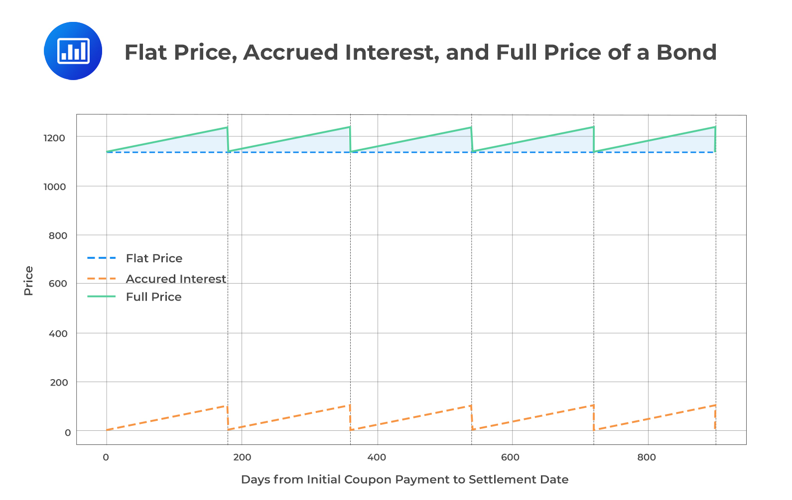
In bond trading, especially when a bond is priced between coupon payment dates, three key components are considered: the flat price, accrued interest, and the full price.

1. Flat Price: The flat price, also known as the quoted or “clean” price, represents the bond’s price without considering any accrued interest.
2. Accrued Interest: Accrued interest is the interest that has accumulated since the last coupon payment but has not yet been paid. It is computed by considering the fraction of the coupon period that has elapsed.Formula for Accrued Interest:\[ AI = \frac{t}{T} \times PMT \]Where:
   • \( t \) = Number of days from the prior coupon payment to the settlement date.
   • \( T \) = Number of days in the coupon period.
   • \( PMT \) = Coupon payment per period.

   The graph below illustrates the relationship between the flat price, accrued interest, and full price of a bond over its entire lifetime, spanning multiple coupon periods.

   1. Flat Price (Dashed Line): Represents the present value of the bond’s future cash flows without considering accrued interest. It remains constant throughout the bond’s lifetime.
   2. Accrued Interest (Dash-Dot Line): Depicts the interest that has accumulated since the last coupon payment. It starts at zero at the beginning of each coupon period and linearly increases until the next coupon payment.
   3. Full Price (Solid Line): The sum of the flat price and accrued interest. It follows the same pattern as accrued interest but starts from the flat price level at the beginning of each coupon period.
   4. Vertical Lines (Dotted Grey Lines): Indicate the end of each coupon period, marking the moments when coupon payments are made.

   The shaded area between the flat price and full price lines visually represents the accrued interest at any given point in time. This graph provides a clear understanding of how these key components of bond pricing interact and evolve over time.

   

1. Full PriceThe full price, or “dirty” price, is the sum of the flat price and the accrued interest. Full Price of a Fixed-Rate Bond is expressed as:\[ PV_{\text{Full}} = \frac{C}{(1 + r)^{1-t/T}} + \frac{C}{(1 + r)^{2-t/T}} + \ldots + \frac{C + FV}{(1 + r)^{N-t/T}} \]Where:
   • \( C\) = Coupon payment per period.
   • \( r \) = Market discount rate per period.
   • \( t \) = Number of days from the prior coupon payment to the settlement date.
   • \( T \) = Number of days in the coupon period.
   • \( N \) = Total number of periods.
   • \( FV \) = Face value of the bond.

Day count conventions specify how days are counted within a period. 30/360 assumes 30 days in a month and 360 days in a year. On the other hand, Actual/Actua uses the actual number of days in a month/year.

Example: Calculating the Flat Price

A certain bond pays semiannual coupons of 2.0% per year on 30 June and 31 December each year, with a face value of 100. The YTM is 2.5%. The bond is purchased and will settle on 15 September, when there will be four coupons remaining until maturity. The flat price of the bond as a percentage of par value, assuming an actual/actual day count, is closest to:

Solution

• PMT = 1.00, i.e., \(2\%\times\frac{100}{2}\).
• r = 0.0125 (2.5% annual market discount rate, divided by 2 for semiannual).
• t = 77 (days from 30 June to 15 September).
• T = 184 (days from 30 June to the next coupon on 31 December).
• FV = 100.
• N = 4 (remaining coupons).

\begin{align*}
PV^{\text{Flat}} & = PV^{\text{Full}} – AI \\
PV^{\text{Full}} & = \left[ \frac{PMT}{(1+r)^1} + \frac{PMT}{(1+r)^2} + \ldots + \frac{PMT+FV}{(1+r)^N} \right] \times \left(1+ r\right)^{\left(\frac{t}{T}\right)} \\
PV^{\text{Full}} & = \left[ \frac{1}{(1.0125)^1} + \frac{1}{(1.0125)^2} + \frac{1}{(1.0125)^3} + \frac{1+100}{(1.0125)^4} \right] \times \left(1.0125\right)^{\left(\frac{77}{184}\right)} = 99.547 \\
AI & = \frac{77}{184} \times 1.00 = 0.418 \\
PV^{\text{Flat}} & = 99.547 – 0.418 = 99.129 \\
\end{align*}

Question

A bond that matures on 1 July 2040 pays semiannual coupons of 2.5% per year and has a face value of 100. The market discount rate is 4.0%. For a trade settlement date of 1 July 2038, the price of the bond as a percentage of par value is closest to:

1. 94.555.
2. 90.018.
3. 97.144.

Solution

The correct answer is C.

Using the given values:

\(PMT=1.25\), i.e., \(\frac{{(2.5\%)}{2} \times 100\)

\(r=0.020\) (4% annual market discount rate, divided by 2 for semiannual)

\(FV=100\)

\(N=4\) (Since payments are made twice a year for 2 years)

Formula for bond price:

\[PV=\frac{C}{{(1+r)^1}} +\frac{C}{{(1+r)^2}} +\frac{C}{{(1+r)^3}} +\frac{{(C+FV)}}{{(1+r)^4}}\]

\[PV=\frac{1.25}{{(1.020)^1}} +\frac{1.25}{{(1.02)^2}} +\cdots+\frac{101.25}{{(1.020)^4}} =97.144\]