




Shortfall Risk, Safety-first Ratio, an ...
Shortfall risk refers to the probability that a portfolio will not exceed the... Read More

The capital asset pricing model, or CAPM, links expected return to systematic risk. The model says that investors should be compensated for bearing market risk, not for risks that can be diversified away. In empirical work, CAPM is often estimated using a simple linear regression of an asset’s excess returns on the market’s excess returns.
This makes CAPM a direct application of simple linear regression. The dependent variable is the asset’s excess return. The independent variable is the market excess return, also called the market risk premium. The slope coefficient is the asset’s estimated beta. The intercept is often interpreted as alpha, or the portion of average excess return not explained by market exposure.
The central skill is to move fluently between the theory and the regression output. A beta estimate is not just a number in a table. It is the slope of the empirical relationship between an asset’s excess return and the market’s excess return.
The CAPM expected return equation is:
$$E(R_i) = R_f + \beta_i [E(R_m) – R_f]$$
Where:
The model can also be written in excess-return form:
$$E(R_i) – R_f = \beta_i [E(R_m) – R_f]$$
Where:
The excess-return form is especially important because empirical CAPM estimation uses excess returns. Instead of regressing the asset’s total return directly on the market’s total return, analysts subtract the risk-free rate from both series.
CAPM is a one-factor model. It explains expected excess return using one source of systematic risk: exposure to the market portfolio. The asset’s beta determines how strongly the asset’s expected return responds to the market risk premium.
An asset with \(\beta = 1.0\) has market-like systematic risk. An asset with \(\beta > 1.0\) is more sensitive to market movements. An asset with \(\beta < 1.0\) is less sensitive. An asset with negative beta tends to move opposite to the market, although such assets are uncommon in ordinary equity portfolios.
$$ \textbf{Table 1: Interpreting Beta Values} \\ \small { \begin{array}{l|l|l|l} \textbf{Beta} & \textbf{Interpretation} & \textbf{Expected} & \textbf{Expected} \\ \textbf{Estimate} & & \textbf{Behavior When} & \textbf{Behavior When} \\ & & \textbf{Market Rises} & \textbf{Market Falls} \\ \hline \beta < 0 & {\text{Negative} \\ \text{market} \\ \text{sensitivity}} & {\text{May} \\ \text{underperform}} & {\text{May provide} \\ \text{downside} \\ \text{offset}} \\ \hline \beta = 0 & {\text{No market} \\ \text{sensitivity}} & {\text{No expected} \\ \text{market-driven} \\ \text{excess return}} & {\text{No expected} \\ \text{market-driven} \\ \text{excess return}} \\ \hline 0 < \beta < 1 & {\text{Defensive} \\ \text{market} \\ \text{sensitivity}} & {\text{Rises less} \\ \text{than market}} & {\text{Falls less} \\ \text{than market}} \\ \hline \beta = 1 & {\text{Market-like} \\ \text{sensitivity}} & {\text{Moves with} \\ \text{market}} & {\text{Moves with} \\ \text{market}} \\ \hline \beta > 1 & {\text{Aggressive} \\ \text{market} \\ \text{sensitivity}} & {\text{Rises more} \\ \text{than market}} & {\text{Falls more} \\ \text{than market}} \end{array} } $$
Table 1 is useful for conceptual interpretation. Beta scales exposure to market risk. It does not measure total risk, liquidity risk, credit risk, or company-specific risk by itself.
To estimate CAPM with observed data, the analyst calculates excess returns:
$$Z_{i,t} = R_{i,t} – R_{f,t}$$
Where:
The market excess return is:
$$Z_{m,t} = R_{m,t} – R_{f,t}$$
Where:
The empirical CAPM regression is:
$$Z_{i,t} = \alpha_i + \beta_i Z_{m,t} + \epsilon_{i,t}$$
Where:
Some texts write the intercept and slope as \(b_0\) and \(b_1\). In CAPM applications, \(b_1\) is the beta estimate, and \(b_0\) is the intercept. If the CAPM holds exactly in expectation, the intercept should be zero. A positive intercept may suggest abnormal performance, but only if it is statistically reliable and economically meaningful.
Figure 1: Empirical CAPM Regression Workflow
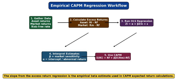
Figure 1 shows the empirical workflow. The analyst starts with asset returns, market returns, and the risk-free rate. Excess returns are calculated for both the asset and the market. A simple linear regression is then estimated. The slope coefficient becomes the beta estimate used in CAPM expected return calculations.
Estimating Beta as a Regression Slope
The OLS slope coefficient can be expressed as:
$$\hat{\beta}_i = \frac{{Cov}(Z_i, Z_m)}{Var(Z_m)}$$
Where:
This formula explains the meaning of beta. Beta is high when an asset’s excess returns strongly co-move with market excess returns relative to the market’s own variance.
Figure 2: CAPM Beta Is Estimated as the Slope in an Excess-Return Regression
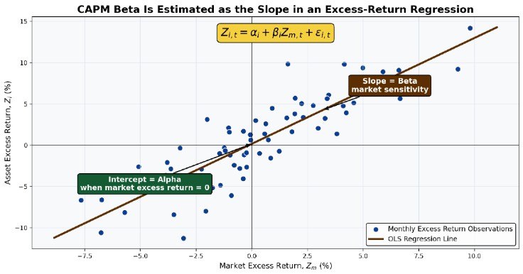
Figure 2 shows a typical CAPM regression. The vertical axis is the asset’s excess return, and the horizontal axis is the market excess return. The slope of the fitted line is beta. The intercept is alpha. A steeper line indicates greater market sensitivity.
Example 1: Calculating Excess Returns for CAPM Estimation
Assume we have the following monthly data for a listed infrastructure stock and a broad market index:
$$ \begin{array}{c|c|c|c}
\textbf{Month} & \textbf{Asset Return} & \textbf{Market Return} & \textbf{Risk-Free Rate} \\ \hline
1 & 2.6\% & 1.8\% & 0.3\% \\ \hline
2 & -1.4\% & -0.8\% & 0.3\% \\ \hline
3 & 3.1\% & 2.2\% & 0.3\% \\
\end{array} $$
Calculate the asset and market excess returns.
Solution
We know that:
$$Z_{i,t} = R_{i,t} – R_{f,t}$$
Where:
The market excess-return formula is:
$$Z_{m,t} = R_{m,t} – R_{f,t}$$
Where:
The calculations are:
$$
\begin{array}{c|c|c}
\textbf{Month} & \textbf{Asset Excess Return} & \textbf{Market Excess Return} \\
\hline
1 & 2.6\% – 0.3\% = 2.3\% & 1.8\% – 0.3\% = 1.5\% \\ \hline
2 & -1.4\% – 0.3\% = -1.7\% & -0.8\% – 0.3\% = -1.1\% \\ \hline
3 & 3.1\% – 0.3\% = 2.8\% & 2.2\% – 0.3\% = 1.9\% \\
\end{array}
$$
The regression would use the asset excess returns as the dependent variable and the market excess returns as the independent variable.
A CAPM regression output typically reports the intercept, the slope, their standard errors, t-statistics, and goodness-of-fit measures such as \(R^2\).
$$ \textbf{Table 2: CAPM Regression Output and Interpretation} \\
\begin{array}{l|l|l}
\textbf{Output Item} & \textbf{Regression Meaning} & \textbf{CAPM Interpretation} \\ \hline
\text{Intercept} & {\text{Predicted asset excess return} \\ \text{when market excess return is zero}} & {\text{Alpha or abnormal excess return} \\ \text{estimate}} \\ \hline
\text{Market excess return coefficient} & \text{Slope coefficient} & {\text{Estimated beta} }\\ \hline
\text{Standard error of beta} & \text{Precision of the beta estimate} & {\text{Used for hypothesis tests} \\ \text{and confidence intervals}} \\ \hline
\text{t-statistic for beta} & \text{Test statistic for beta hypothesis} & {\text{Tests whether beta differs from} \\ \text{a hypothesized value}} \\ \hline
R^2 & {\text{Share of variation in asset} \\ \text{excess returns explained by} \\ \text{market excess returns}} & {\text{Proportion of asset excess-return} \\ \text{variance explained by market} \\ \text{exposure}}
\end{array} $$
Table 2 highlights a common exam trap. The beta is the coefficient on the market excess return, not the standard error, t-statistic, or \(R^2\). The \(R^2\) tells us how much of the asset excess-return variation is explained by the market excess return.
Example 2: Identifying Beta, Alpha, and \(\bf{R^2}\)
Consider the following regression output for a renewable-energy stock, using 60 monthly observations:
$$ \begin{array}{l|c}
\textbf{Regression Statistic} & \textbf{Value} \\
\hline
R^2 & 0.64 \\ \hline
\text{Standard error of estimate} & 4.10\% \\ \hline
\text{Observations} & 60 \\
\end{array}
$$
$$ \begin{array}{l|r|r|r}
\textbf{Coefficient} & \textbf{Estimate} & \textbf{Standard Error} & \textbf{t-Statistic} \\ \hline
\text{Intercept} & 0.0020 & 0.0040 & 0.50 \\ \hline
\text{Market excess return} & 1.35 & 0.20 & 6.75 \\
\end{array}
$$
The regression equation is:
$$ Z_{i,t} = 0.0020 + 1.35Z_{m,t} + \epsilon_{i,t} $$
The estimated beta is 1.35, because beta is the slope coefficient on the market excess return. The estimated intercept, or alpha, is 0.20% per month. The \(R^2\) of 0.64 means that 64% of the variation in the stock’s monthly excess returns is explained by market excess returns. The remaining 36% is not explained by the market factor in this one-factor model.
The t-statistic of 6.75 suggests that the beta estimate is statistically different from zero in this sample, assuming the regression assumptions are sufficiently reliable.
After estimating beta, the analyst can calculate the expected return using the CAPM equation:
$$ E(R_i) = R_f + \hat{\beta}_i [E(R_m) – R_f] $$
Where:
This is where regression output becomes a valuation input. Beta connects the asset to the market risk premium. The higher the beta, the larger the expected excess return demanded by investors.
Figure 3: Beta Scales the Asset’s Expected Excess Return for a Given Market Risk Premium
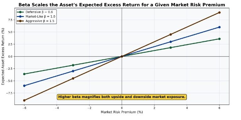
Figure 3 shows how beta scales expected excess return. When the market risk premium is positive, higher-beta assets have higher expected excess returns. When the market risk premium is negative, higher-beta assets are expected to fall more sharply. Beta magnifies exposure to broad market movements.
Example 3: Calculating a CAPM Expected Return
Let’s say a technology stock has an estimated beta of 1.40. The risk-free rate is 3.00%, and the expected market return is 8.50%.
Calculate the stock’s expected return using CAPM.
Solution
Recall the CAPM equation:
$$E(R_i) = R_f + \hat{\beta}_i [E(R_m) – R_f]$$
Where:
Substitute the values:
$$E(R_i) = 3.00\% + 1.40(5.50\%)$$
$$E(R_i) = 3.00\% + 7.70\% = 10.70\%$$
The CAPM expected return is 10.70%. The stock has a higher expected return than the market because its beta exceeds 1.0.
The CAPM regression can also be used to estimate the change in the asset’s excess return for a change in the market excess return:
$$\Delta Z_i = \hat{\beta}_i \Delta Z_m$$
Where:
This calculation focuses only on excess return. The risk-free rate should not be added unless the question asks for the asset’s total expected return and provides the relevant risk-free rate.
Example 4: Calculating the Effect of a Change in Market Risk Premium
Suppose a consumer-discretionary stock has an estimated beta of 1.25. The market risk premium increases by 0.80 percentage points. The risk-free rate does not change. Estimate the change in the stock’s expected excess return.
Solution
We know that:
$$\Delta Z_i = \hat{\beta}_i \Delta Z_m$$
Where:
Calculate:
$$\Delta Z_i = 1.25(0.80\%) = 1.00\%$$
The stock’s expected excess return increases by 1.00 percentage point. The unchanged risk-free rate is not added because the question asks only for the change in excess return.
A beta estimate is based on sample data. It is therefore subject to estimation error. A confidence interval for beta can be calculated as:
$$\hat{\beta}_i \pm t_{\alpha/2} s_{\hat{\beta}}$$
Where:
A narrow interval indicates a more precise beta estimate. A wide interval indicates greater estimation uncertainty.
Example 5: Constructing a Confidence Interval for Beta
Assume a healthcare stock has an estimated beta of 0.82. The standard error of beta is 0.14, and the relevant two-tailed 95% critical t-value is 2.00.
Construct the 95% confidence interval for beta.
Solution
Start with the confidence interval formula:
$$\hat{\beta}_i \pm t_{\alpha/2} s_{\hat{\beta}}$$
Where:
Calculate the margin of error:
$$2.00(0.14) = 0.28$$
The confidence interval is:
$$0.82 \pm 0.28 = [0.54, 1.10]$$
The 95% confidence interval is [0.54, 1.10]. Because the interval includes 1.0, the analyst cannot conclude from this interval alone that the stock’s beta is statistically different from the market beta of 1.0 at the 5% level.
The t-statistic for testing beta is:
$$t = \frac{\hat{\beta}_i – \beta_0}{s_{\hat{\beta}}}$$
Where:
The common hypotheses are:
$$ \begin{align*} H_0& : \beta_i = \beta_0 \\ H_a & : \beta_i \neq \beta_0 \end{align*} $$
Where:
The analyst rejects the null hypothesis when the t-statistic is sufficiently extreme or when the p-value is below the chosen significance level.
Example 6: Testing Whether Beta Is Greater Than One
Assume a growth stock has an estimated beta of 1.32 with a standard error of 0.16. The analyst wants to test whether the beta is greater than 1.0 at the 5% significance level. The one-sided critical t-value is 1.67.
The hypotheses are:
$$ \begin{align*} H_0 & : \beta_i \leq 1.0 \\ H_a & : \beta_i > 1.0 \end{align*} $$
Now quote the t-statistic:
$$t = \frac{\hat{\beta}_i – \beta_0}{s_{\hat{\beta}}}$$
Where:
Calculate:
$$t = \frac{1.32 – 1.00}{0.16} = 2.00$$
Because 2.00 is greater than the one-sided critical value of 1.67, the analyst rejects the null hypothesis. The evidence supports the conclusion that the stock’s beta is greater than 1.0.
In a CAPM regression, \(R^2\) measures the proportion of variation in the asset’s excess returns explained by variation in market excess returns.
$$R^2 = \frac{SSR}{SST}$$
Where:
A high \(R^2\) means that market movements explain a large share of the asset’s excess-return variation. A low \(R^2\) means that much of the asset’s variation is not explained by the market factor.
\(R^2\) should not be confused with beta. Beta is the slope. \(R^2\) is the explained variation share. A stock can have a high beta and a low \(R^2\) if it is highly sensitive to the market when it moves with the market but also has large idiosyncratic movements.
Example 7: Interpreting CAPM R2
Consider two stocks:
$$\begin{array}{l|c|c}
\textbf{Stock} & \textbf{Beta} & \bf{R^2} \\
\hline
\text{A} & 1.30 & 0.78 \\ \hline
\text{B} & 1.30 & 0.22 \\
\end{array}$$
Both stocks have the same beta. Both are estimated to have the same sensitivity to market excess returns. But the market explains 78% of Stock A’s excess-return variation and only 22% of Stock B’s excess-return variation.
Stock B likely has more firm-specific or non-market variation. The same beta does not imply the same total risk, and it does not imply the same goodness-of-fit.
CAPM is widely used because it is simple, intuitive, and connected to the idea of systematic risk. It is also limited.
First, expected returns are not directly observable, so analysts use realized returns as proxies. Second, the true market portfolio is unobservable, so analysts use broad market indexes as proxies. Third, beta estimates depend on the sample period, return frequency, risk-free rate proxy, and market index proxy. Fourth, CAPM is a one-factor model and ignores other sources of return such as size, value, momentum, quality, liquidity, and macroeconomic exposures.
These limitations do not make CAPM useless. They mean that CAPM outputs should be interpreted as estimates rather than truths.
$$ \textbf{Table 3: CAPM Regression Traps} \\
\begin{array}{l|l|l}
\textbf{Trap} & \textbf{Why It Is Wrong} & \textbf{Correct Interpretation} \\ \hline
\text{Treating beta as total risk} & {\text{Beta captures systematic market} \\ \text{sensitivity only}} & {\text{Total risk also includes} \\ \text{idiosyncratic risk}} \\ \hline
\text{Treating } R^2 \text{ as beta} & R^2 \text{ is explained variation, not slope} & {\text{Beta is the coefficient on} \\ \text{market excess return}} \\ \hline
\text{Adding the risk-free rate when} & \text{Excess-return changes exclude the} & \text{Use } \Delta Z_i = \beta \Delta Z_m \\
\text{calculating a change in excess return} & \text{risk-free rate unless it changes} & \\ \hline
\text{Treating a positive alpha as proof} & \text{Alpha must be statistically and} & \text{Test the intercept and consider} \\
\text{of skill} & \text{economically evaluated} & \text{model limitations} \\ \hline
\text{Assuming beta is permanent} & \text{Beta depends on the sample and} & \text{Re-estimate and interpret in} \\
& \text{business risk} & \text{context} \\
\end{array}
$$
Table 3 summarizes the most common interpretation errors. Many exam questions test whether a candidate can distinguish the slope, the intercept, the \(R^2\), and the expected return calculation.
Several practical principles follow:
Question
A regression of a manufacturing stock’s monthly excess returns on market excess returns produces the following output:
$$
\begin{array}{l|c|c}
\textbf{Coefficient} & \textbf{Estimate} & \textbf{Standard Error} \\ \hline
\text{Intercept} & 0.0015 & 0.0020 \\ \hline
\text{Market excess return} & 1.18 & 0.12
\end{array}
$$The risk-free rate is 3.00%, and the expected market return is 8.00%. Based on the regression estimate, the stock’s CAPM expected return is closest to:
- 5.90%
- 8.90%
- 9.35%
Solution
The correct answer is B.
The beta estimate is the slope coefficient on the market excess return. Therefore:
$$\hat{\beta} = 1.18$$
Now recall the CAPM expected return formula:
$$E(R_i) = R_f + \hat{\beta}_i [E(R_m) – R_f]$$
Where:
- \(E(R_i)\) is the expected return on the manufacturing stock
- \(R_f = 3.00\%\) is the risk-free rate
- \(\hat{\beta}_i = 1.18\) is the estimated beta
- \(E(R_m) = 8.00\%\) is the expected market return
- \(E(R_m) – R_f = 8.00\% – 3.00\% = 5.00\%\) is the expected market risk premium
Substitute the values:
$$ \begin{align*} E(R_i) & = 3.00\% + 1.18(5.00\%) \\
E(R_i) & = 3.00\% + 5.90\% = 8.90\% \end{align*} $$The stock’s CAPM expected return is 8.90%.
A is incorrect because it gives only the beta-scaled market risk premium, \(1.18(5.00\%) = 5.90\%\), and omits the risk-free rate.
C is incorrect because it incorrectly adds the regression intercept to the CAPM expected return after already using the CAPM formula. The intercept may be interpreted as alpha in a regression, but the standard CAPM expected return calculation uses the risk-free rate plus beta times the expected market risk premium.
Master CFA Level I Quantitative Methods and Portfolio Management concepts, including CAPM regression, alpha, beta, market risk premium, expected return, and exam-style practice questions with study notes, mock exams, and video lessons.






Get Ahead on Your Study Prep This Cyber Monday! Save 35% on all CFA® and FRM® Unlimited Packages. Use code CYBERMONDAY at checkout. Offer ends Dec 1st.