Financial Returns Explained: Price Return, Income Return, Total Return, and Compounding

Introduction to Financial Returns

A return measures the change in an investor’s economic position over a specified period. At first glance, the concept seems straightforward: compare the investment’s value at the end of the period with its value at the beginning. In practice, however, investments generate different combinations of price changes, cash distributions, and contractual payoffs. A useful return measure must therefore align both with the instrument being analyzed and the period over which performance is assessed.

For example, a growth company’s shares may generate most of their return through an increase in market price. A mature dividend-paying company may provide a meaningful portion of return through cash dividends. A bond may combine a changing market price with periodic coupon payments. The same return framework can also be applied to newer investment themes, such as digital-asset funds, energy-transition infrastructure, and technology-focused exchange-traded funds, even though their cash-flow patterns may differ.

The central question throughout this learning outcome is not merely, “What number did the investment earn?” It is also, “What produced the return, over what period was it measured, and how should it be interpreted?”

Financial Assets, Financial Instruments, and Financial Indicators

A financial asset is a claim or store of financial value held by an investor. Cash, equity ownership, debt claims, and hybrid securities are common examples. An equity investment represents an ownership interest, while a bond represents a claim on the issuer’s promised payments.

A financial instrument is a standardized and tradable form through which a financial claim is issued or transferred. Shares, bonds, options, futures, and other contracts package particular cash-flow or payoff patterns into securities that can be bought and sold.

A financial indicator is an observable measure of value or market conditions rather than a directly tradable asset. Interest rates, exchange rates, and market indexes are examples. An indicator does not itself make a cash distribution, although a security or derivative may be designed to provide exposure to movements in that indicator.

$$ \textbf{Table 1: Financial Assets, Financial Instruments, and Financial Indicators} \\
\small { \begin{array}{l|c|c|c}
\textbf{Category} & \textbf{Main } & \textbf{Common } & \textbf{Return } \\
{} & \textbf{Characteristic} & \textbf{Examples} & \textbf{Implication} \\ \hline
\text{Financial asset} & {\text{Represents financial} \\ \text{value or a claim}} & {\text{Cash, equity, debt,} \\ \text{hybrid security}} &
{\text{May produce price} \\ \text{changes, distributions,} \\ \text{or both}} \\ \hline
\text{Financial instrument} &
{\text{Standardizes and} \\ \text{packages a financial} \\ \text{claim or payoff}} &
{\text{Share, bond, option,} \\ \text{futures contract}} &
{\text{Return depends on the} \\ \text{instrument’s contractual} \\ \text{cash flows and market} \\ \text{value}} \\ \hline
\text{Financial indicator} &
{\text{Measures value or} \\ \text{market conditions but is} \\ \text{not itself a} \\ \text{cash-flow-producing} \\ \text{asset}} &
{\text{Exchange rate, interest} \\ \text{rate, market index}} &
{\text{An investor generally} \\ \text{obtains exposure} \\ \text{through another} \\ \text{instrument}}
\end{array} } $$

Table 1 highlights why the nature of the investment matters. A market index may rise by 8%, but an investor cannot receive that index return without holding an instrument that tracks or replicates it. Similarly, a bond’s coupon payment and price movement must both be considered when evaluating the investor’s performance.

How an Investment Generates Return

Figure 1: How an Investment Generates Total Return

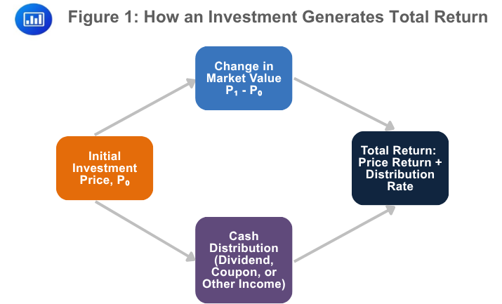
Figure 1 separates the two basic sources of investment return. The first is the change in market value between the beginning and end of the holding period. The second is any cash distribution received while the investment is held. Combining the two gives total return. This decomposition is useful because two investments can have the same total return while relying on very different sources. One may depend almost entirely on price appreciation, while another may deliver a large part of its return through dividends or coupon income.

Price Return

The price return, also called the capital appreciation return, measures the percentage change in the asset’s market price over the holding period:

$$ r_{\text{price}}=\frac {P_1-P_0}{P_0} $$

Where:

• \(r_{\text{price}}\) is the price return over the holding period
• \(P_0\) is the price at the beginning of the holding period
• \(P_1\) is the price at the end of the holding period

A positive price return indicates appreciation; a negative price return indicates depreciation. The price return excludes dividends, coupons, and other cash distributions.

Capital Distribution Return

The capital distribution return measures cash income received during the holding period relative to the initial investment:

$$ r_{\text{distribution}}=\frac {Inc}{P_0} $$

Where:

• \(r_{\text{distribution}}\) is the capital distribution return
• \(Inc\) is the cash income received during the holding period
• \(P_0\) is the beginning price or initial amount invested

For equity, the capital distribution return is commonly called the dividend yield. For a bond, the annual coupon divided by the bond’s beginning market price is commonly called the current yield. The denominator is the market price paid, not necessarily the security’s face value.

Total Return

The total return combines the price return and the capital distribution return:

$$ r=r_{\text{price}}+r_{\text{distribution}}=\frac {P_1-P_0+Inc}{P_0} $$

Where:

• \(r\) is the total holding-period return
• \(r_{\text{price}}\) is the price return
• \(r_{\text{distribution}}\) is the capital distribution return
• \(P_0 \) is the beginning price
• \(P_1\) is the ending price
• \(Inc\) is the cash distribution received during the period

The total return is the appropriate measure when the investor receives both a change in market value and cash income. Focusing on only one component can produce a misleading assessment. A bond’s price might fall slightly during a year, for example, while coupon income allows the investor to earn a positive total return.

Example 1: Calculating an Equity Investment’s Total Return

Suppose we want to calculate the one-year total return on shares of an AI-infrastructure company. An investor buys the shares for USD 84.00, receives a dividend of USD 1.80, and sells the shares one year later for USD 91.50. This is how to approach the problem:

Start by quoting the formula:

$$ r=\frac {P_1-P_0+Inc}{P_0} $$

Where:

• \(P_0\)=USD 84.00, the purchase price
• \(P_1\)=USD 91.50, the sale price
• \(Inc\)=USD 1.80, the dividend received
• \(r\) is the total return to be calculated

Calculate the price return:

$$ r_{\text{price}}=\frac {91.50-84.00}{84.00}=8.93\% $$

Calculate the dividend yield:

$$ r_{\text{distribution}}=\frac {1.80}{84.00}=2.14\% $$

Finally, combine the two components:

$$ r=8.93\%+2.14\%=11.07\% $$

The investor earned a total return of 11.07%. Most of the return came from the increase in the share price, while the dividend provided an additional 2.14 percentage points.

Example 2: Interpreting a Bond’s Price Return and Current Yield

Suppose we wanted to calculate the total return on a corporate bond purchased at 97.60 per 100 of face value. One year later, the bond is priced at 99.20 and has paid a coupon of 4.20 per 100 of face value. This is how we proceed:

The formula is given as:

$$ r=\frac {P_1-P_0+Inc}{P_0} $$

Where:

• \(P_0=97.60\), the bond’s initial market price
• \(P_1=99.20\), the bond’s ending market price
• \(Inc=4.20\), the coupon received
• \(r\) is the bond’s total return

The price return is:

$$ r_{\text{price}}=\frac {99.20-97.60}{97.60}=1.64\% $$

The current yield is:

$$ r_{\text{distribution}}=\frac {4.20}{97.60}=4.30\% $$

The total return is:

$$ r=1.64\%+4.30\%=5.94\% $$

The bond earned a total return of 5.94%. The example also shows why the coupon rate and current yield should not be considered identical. The coupon is stated relative to the face value, whereas the current yield is based on the bond’s market price.

Expected and Actual Returns

An expected return, also called an ex ante return, is estimated before the investment outcome is known. It may be based on valuation models, historical evidence, economic forecasts, or scenario analysis. Expected return is a decision-making input, not a guarantee.

An actual return, also called an ex post return, is measured after the holding period has ended. It reflects what the investor actually experienced. Unexpected changes in interest rates, inflation, regulation, business conditions, or market sentiment can cause actual return to differ materially from expected return.

The distinction is central to investment risk. Investors commit capital based on expected returns, but wealth changes with realized outcomes. When the range of possible actual returns is wide, investors generally require greater compensation for bearing uncertainty.

Realized and Unrealized Returns

An unrealized return arises when the market value of an investment changes while the investor continues to hold it. It is often described as a paper gain or paper loss because the position has not yet been sold.

A realized return occurs when the investor sells the investment or receives a cash distribution. Dividends and coupon payments are normally realized when received. A price gain or loss becomes realized when the security is sold.

This distinction matters for performance reporting, liquidity planning, and taxation. A portfolio may show a large unrealized gain, but that gain can change before the position is sold. Conversely, a realized distribution has already increased the investor’s cash holdings.

$$ \textbf{Table 2: Comparison of Important Return Distinctions} \\ \small { \begin{array}{l|l|l|l} \textbf{Return} & \textbf{First} & \textbf{Second} & \textbf{Key} \\ {} & \textbf{Concept} & \textbf{Concept} & \textbf{Interpretation} \\ \hline {\text{Expected} \\ \text{versus} \\ \text{actual}} & {\text{Forecast} \\ \text{before} \\ \text{the outcome}} & {\text{Observed} \\ \text{after} \\ \text{the outcome}} & {\text{Investment} \\ \text{decisions use} \\ \text{expectations,} \\ \text{but wealth} \\ \text{changes} \\ \text{according to} \\ \text{actual} \\ \text{results}} \\ \hline {\text{Unrealized} \\ \text{versus} \\ \text{realized}} & {\text{Market-value} \\ \text{change on} \\ \text{an open} \\ \text{position}} & {\text{Gain, loss,} \\ \text{or} \\ \text{distribution} \\ \text{already} \\ \text{crystallized}} & {\text{Unrealized} \\ \text{performance} \\ \text{can change} \\ \text{before} \\ \text{sale}} \\ \hline {\text{Price} \\ \text{versus} \\ \text{distribution}} & {\text{Change in} \\ \text{market} \\ \text{price}} & {\text{Cash income} \\ \text{received}} & {\text{Both} \\ \text{components} \\ \text{may be} \\ \text{needed to} \\ \text{evaluate} \\ \text{total return}} \\ \hline {\text{Single-period} \\ \text{versus} \\ \text{multi-period}} & {\text{Performance} \\ \text{over one} \\ \text{interval}} & {\text{Performance} \\ \text{across} \\ \text{several} \\ \text{linked} \\ \text{intervals}} & {\text{Multi-period} \\ \text{analysis} \\ \text{must} \\ \text{account for} \\ \text{compounding}} \\ \end{array} } $$

 

Table 2 brings together distinctions that candidates often confuse. The concepts are related but not interchangeable. An expected price gain, for instance, is neither an actual return nor a realized return until the relevant events occur.

Single-Period and Multi-Period Returns

A single-period return measures performance over one clearly defined interval, such as one day, one month, one quarter, or one year. The beginning and ending values must correspond to that same interval.

A multi-period return summarizes performance over several consecutive intervals. Because each period’s ending value becomes the next period’s starting value, returns compound through time. This compounding effect is why multi-period performance cannot generally be summarized by simply adding or averaging returns without considering the purpose of the calculation.

For practical calculations, analysts commonly use the closing price on the final trading day of one period as the beginning price for the next period. Monthly returns, for example, compare the closing price at the end of the previous month with the closing price at the end of the current month.

Arithmetic Mean Return

The arithmetic mean return is the simple average of periodic returns:

$$
\overline{r}_i=\frac{1}{T}\sum_{t=1}^{T} r_{i,t}
$$

Where:

• \(r_i\) is the arithmetic mean return for asset \(i\)
• \(T\) is the number of holding periods
• \(r_{i,t}\) is the return on asset \(i\) during period \(t\)
• The summation operator indicates that the periodic returns are added from period 1 through period \(T\)

The arithmetic mean describes the average one-period outcome when each observation receives equal weight. It is often useful for estimating an average return for a single future period, but it does not measure the compound growth rate actually earned over several periods.

Geometric Mean Return

The geometric mean return is the constant periodic rate that compounds to the same ending wealth as the observed sequence of returns:

$$
\overline{{r}}_{G,i}=\left[\prod_{t=1}^{T}(1+r_{i,t})\right]^{\frac{1}{T}}-1
$$

Where:

• \(\overline{r}_{G,i}\) = geometric mean return for asset \(i\)
• \(T\) = number of holding periods
• \(r_{i,t}\) = return during period \(t\)
• \(\prod\) denotes the product operator, indicating that the periodic growth factors are multiplied.
• \(1+r_{i,t}\) = growth factor for period \(t\)

The geometric mean is the more appropriate measure of historical compound performance because it accounts for the effect of compounding. It recognizes that losses reduce the capital base on which subsequent returns are earned.

Example 3: Comparing Arithmetic and Geometric Mean Returns

Suppose we wish to summarize the annual performance of a cybersecurity fund that earned 24% in Year 1, lost 12% in Year 2, and earned 9% in Year 3. We want both the average one-year return and the compound annual growth rate. We solve the problem as follows:

Apply the formula:

$$ \begin{align*}
\overline{r} & =\frac{1}{T}\sum_{t=1}^{T}r_t \\
\overline{r}_{G} & =\left[\prod_{t=1}^{T}(1+r_t)\right]^{\frac{1}{T}}-1
\end{align*} $$

Where:

• \(T=3\), the number of annual observations
• \(r_1=24\%\), \(r_2=-12\%\), and \(r_3=9\%\)
• \(\overline{r}\) is the arithmetic mean return
• \(\overline{r}_{G}\) is the geometric mean return

The arithmetic mean is:

$$
\overline{r}=\frac{24\%-12\%+9\%}{3}=7.00\%
$$

The geometric mean is:

$$
\overline{r}_{G}=\left[(1.24)(0.88)(1.09)\right]^{\frac{1}{3}}-1=5.95\%
$$

The arithmetic mean is 7.00%, while the geometric mean is 5.95%. The geometric mean is lower because the sequence
contains variable returns, including a loss. It is the appropriate measure of the fund’s annualized compound growth over the three-year period.

The Arithmetic-Geometric Mean Relationship

When periodic returns are identical, the arithmetic and geometric means are equal. When returns vary, the geometric mean is lower. The difference between the two measures becomes wider as return variability increases.

$$ \textbf{Table 3: Return Variability and the Arithmetic-Geometric Mean Gap} \\
{
\begin{array}{l|c|c}
\textbf{Three-Year Return Path} &
\textbf{Arithmetic Mean} &
\textbf{Geometric Mean}
\\ \hline
10\%,\,10\%,\,10\% &
10.00\% &
10.00\%
\\ \hline
30\%,\,-10\%,\,10\% &
10.00\% &
8.77\%
\\ \hline
50\%,\,-30\%,\,10\% &
10.00\% &
4.92\%
\end{array}
}
$$

Every return path in Table 3 has the same arithmetic mean, but the compound outcomes differ sharply. Greater variability produces a lower geometric mean
because losses and gains are not symmetric in wealth terms. A 50% loss, for example, requires a 100% gain to restore the original value.

This relationship is sometimes described as volatility drag. It does not mean that volatility is a separate cash expense. Rather, it
describes how uneven returns reduce compound growth relative to the arithmetic average.

Annualizing Returns

Returns measured over different periods should be placed on a common time basis before being compared. If a periodic return is assumed to repeat and compound for \(c\) periods per year, the annualized return is:

$$ r_{\text{annualized}}=(1+r_{\text{period}})^c-1 $$

Where:

• \(r_{\text{annualized}}\) is the annualized return
• \(r_{\text{period}}\) is the return earned over one measurement period
• \(c\) is the number of such periods in one year

The inverse relationship converts an annual return into an equivalent periodic return:

$$ r_{\text{period}}=(1+r_{\text{annualized}})^{\frac{1}{c}}-1 $$

Where:

• \(r_{\text{period}}\) is the periodic return
• \(r_{\text{annualized}}\) is the annual return
• \(c\) is the number of compounding periods in one year

Annualization improves comparability, but introduces an important assumption: the observed periodic return can be repeated at the same rate. This assumption is particularly questionable when a short period contains an unusually strong rally, a sharp selloff, or a one-time event.

Example 4: Annualizing a Four-Month Return

Suppose we want to compare a four-month return of 5.2% on an energy-storage fund with annual returns reported for other funds. We therefore need to annualize the four-month result. We proceed as follows:

Start by quoting the formula:

$$
r_{\text{annualized}}=\left(1+r_{\text{period}}\right)^c-1
$$

Where:

• \(r_{\text{period}} = 5.2\%\), the return earned over four months.
• \(c = 3\), because three four-month periods fit into one year.
• \(r_{\text{annualized}}\) is the return to be calculated.

Substituting the information:

$$
r_{\text{annualized}}=(1.052)^3-1=16.43\%
$$

The annualized return is 16.43%. This result is useful for comparison, but it should not be interpreted as a forecast that the fund will
necessarily earn 16.43% over the next twelve months. It assumes that the four-month performance can be repeated twice more at the same compound rate.

Continuously Compounded Returns

A continuously compounded price return, also called a logarithmic return, is the natural logarithm of the ending-to-beginning price ratio. If cash distributions are part of the return, the analyst should use an appropriately adjusted total-return series.

$$
\widetilde{r}_{t,t+1}
=\ln\!\left(\frac{P_{t+1}}{P_t}\right)
=\ln\!\left(1+r_{t,t+1}\right)
$$

Where:

• \(\widetilde{r}_{t,t+1}\) is the continuously compounded return from time \(t\) to time \(t+1\).
• \(P_t\) is the price at time \(t\).
• \(P_{t+1}\) is the price at time \(t+1\).
• \(r_{t,t+1}\) is the corresponding simple holding-period return.
• \(\ln(\cdot)\) is the natural logarithm.

The continuously compounded return can be converted back to a simple return:

$$
r_{t,t+1}=e^{\widetilde{r}_{t,t+1}}-1
$$

Where:

• \(e\) is the base of the natural logarithm.
• \(\widetilde{r}_{t,t+1}\) is the continuously compounded return.
• \(r_{t,t+1}\) is the simple holding-period return.

The most useful property of continuously compounded returns is that they are additive through time:

$$
\widetilde{r}_{0,T} = \sum_{t=0}^{T-1}\widetilde{r}_{t,t+1} = \ln\!\left(\frac{P_T}{P_0}\right)
$$

Where:

• \(\widetilde{r}_{0,T}\) is the continuously compounded return over the complete period.
• \(\widetilde{r}_{t,t+1}\) is the continuously compounded return for each subperiod.
• \(P_0\) is the initial price.
• \(P_T\) is the final price.
• The summation operator indicates that the subperiod logarithmic returns are added.

Simple returns must be compounded by multiplying growth factors. Log returns can instead be added, which is convenient in time-series analysis and quantitative modeling.

Example 5: Calculating and Combining Continuously Compounded Returns

Suppose we wish to calculate the six-month continuously compounded return on a technology-services share whose price rises from USD 58.00 to USD 63.50. The price is USD 60.50 after the first three months. We also want to confirm that the two three-month log returns add to the full six-month log return. This is how to approach the problem:

We use the formula:

$$
\widetilde{r}_{0,2} = \ln\!\left(\frac{P_2}{P_0}\right)
$$

$$
\widetilde{r}_{0,2} = \widetilde{r}_{0,1} + \widetilde{r}_{1,2}
$$

Where:

• \(P_0=\text{USD }58.00\), the beginning price.
• \(P_1=\text{USD }60.50\), the price after three months.
• \(P_2=\text{USD }63.50\), the price after six months.
• \(\widetilde{r}_{0,1}\) is the first three-month continuously compounded return.
• \(\widetilde{r}_{1,2}\) is the second three-month continuously compounded return.
• \(\widetilde{r}_{0,2}\) is the full six-month continuously compounded return.

The direct six-month calculation is:

$$
\widetilde{r}_{0,2} = \ln\!\left(\frac{63.50}{58.00}\right) = 9.06\%
$$

The two subperiod returns are:

$$
\widetilde{r}_{0,1} = \ln\!\left(\frac{60.50}{58.00}\right) = 4.22\%
$$

$$
\widetilde{r}_{1,2} = \ln\!\left(\frac{63.50}{60.50}\right) = 4.84\%
$$

Adding the subperiod logarithmic returns:

$$
4.22\%+4.84\%=9.06\%
$$

The result matches the direct calculation. This confirms the additive property of continuously compounded returns.

Interpretation and Evaluation

Several practical principles follow:

• A return should always be linked to a clearly defined holding period.
• Total return should include cash distributions when they are part of the investor’s payoff.
• Arithmetic mean return describes an average one-period observation; geometric mean return describes compound growth.
• Annualized returns improve comparability but can exaggerate short-term performance when the repetition assumption is unrealistic.
• Continuously compounded returns are useful because they are additive through time.
• Expected, actual, realized, and unrealized returns answer different questions and should not be used interchangeably.

Question

An equity fund reports annual total returns of 16.0%, -8.0%, and 12.0% over three consecutive years. Its geometric mean annual return is closest to:

1. 5.40%
2. 6.13%
3. 6.67%

Answer Explanation

The correct answer is B.

We apply the formula:

$$
\overline{r}_{G} =\left[\prod_{t=1}^{T}(1+r_t)\right]^{\frac{1}{T}}-1
$$

Where:

• \(\overline{r}_{G}\) is the geometric mean annual return.
• \(T=3\) is the number of annual observations.
• \(r_1=16.0\%\), \(r_2=-8.0\%\), and \(r_3=12.0\%\) are the annual returns.
• The product operator indicates that the annual growth factors are multiplied.

Substituting the returns:

$$
\overline{r}_{G} = \left[(1.16)(0.92)(1.12)\right]^{\frac{1}{3}}-1 = 6.13\%
$$

The arithmetic mean does not capture the compound effect of the return sequence.