Simple Linear Regression in Finance: Least Squares, Intercepts, Slopes, and Interpretation

Why Linear Regression Matters in Finance

Investment professionals rarely observe relationships directly. They observe data: asset returns, earnings growth, inflation, interest rates, credit spreads, valuation multiples, factor exposures, transaction costs, fund flows, and other market variables. Linear regression gives the analyst a structured way to ask whether one variable helps explain another.

In finance, regression is often used to estimate sensitivities, test investment ideas, interpret portfolio behavior, and make forecasts. A risk analyst may regress a fund’s excess return on the market’s excess return to estimate beta. An equity analyst may test whether operating margins are related to revenue growth. A macro strategist may examine whether changes in bond yields are associated with changes in inflation expectations. In each case, the goal is not merely to draw a line through data. The goal is to quantify a relationship and interpret it with economic discipline.

Simple linear regression examines the relationship between one dependent variable and one independent variable. It is called “simple” because there is only one explanatory variable. It is linear because the model fits a straight-line relationship between the two variables.

Dependent and Independent Variables

The dependent variable, usually denoted as Y, is the variable the analyst is trying to explain or predict. The independent variable, usually denoted as X, is the variable used to explain changes in Y.

The language matters. If an analyst says that monthly fund excess returns are regressed on monthly market excess returns, the fund’s excess return is the dependent variable and the market’s excess return is the independent variable. The model is trying to explain the fund’s return behavior using market behavior.

$$ \textbf{Table 1: Dependent and Independent Variables in Financial Regression} \\
\begin{array}{l|l|l|l}
\textbf{Research Question} & \textbf{Dependent Variable, Y} & \textbf{Independent Variable, X} & \textbf{Interpretation Focus} \\ \hline
\text{How sensitive is a stock} & \text{Stock excess return} & \text{Market excess return} & \text{Market exposure or beta} \\
\text{to the market?} & & & \\ \hline
\text{Do valuation multiples} & \text{Future stock return} & \text{Beginning valuation} & \text{Predictive relationship} \\
\text{explain future returns?} & & \text{multiple} & \\ \hline
\text{Are credit spreads related} & \text{Credit spread change} & \text{Expected default rate} & \text{Credit-risk sensitivity} \\
\text{to default expectations?} & & \text{change} & \\ \hline
\text{Does revenue growth} & \text{Change in operating} & \text{Revenue growth} & \text{Operating leverage} \\
\text{explain margin} & \text{margin} & & \\
\text{expansion?} & & & \\ \hline
\text{Do fund flows follow} & \text{Net fund flow} & \text{Prior-period return} & \text{Investor behavior} \\
\text{recent performance?} & & & \\
\end{array} $$

Table 1 highlights the core structure. Regression is not only a statistical exercise. The dependent and independent variables must be chosen in a way that makes economic sense.

Simple Linear Regression Model

The simple linear regression model can be written as:

$$
Y_i = b_0 + b_1 X_i + \epsilon_i, \quad i = 1, 2, \dots, n
$$

Where:

• \(Y_i\) is the observed value of the dependent variable for observation \(i\)
• \(X_i\) is the observed value of the independent variable for observation \(i\)
• \(b_0\) is the intercept of the population regression line
• \(b_1\) is the slope coefficient of the population regression line
• \(\epsilon_i\) is the error term for observation \(i\)
• \(n\) is the number of paired observations

The intercept, \(b_0\), is the value of \(Y\) when \(X\) equals zero. In many finance applications, the intercept is meaningful only if zero is a realistic value for \(X\). If zero is outside the relevant range of the data, the intercept may be a necessary part of the line but not a useful economic prediction.

The slope coefficient, \(b_1\), measures the expected change in \(Y\) for a one-unit increase in \(X\). The unit must be interpreted carefully. If \(X\) is expressed in decimals, a change from 0.04 to 0.05 is a one-percentage-point change but not a one-unit change. If \(X\) is expressed in percentage points, then the coefficient is interpreted directly per percentage-point change.

The error term, \(\epsilon_i\), captures the part of \(Y_i\) that the model does not explain. It includes omitted variables, measurement noise, random shocks, nonlinear effects, and any other influence not captured by the single independent variable.

Estimated Regression Equation

In practice, the analyst does not know the true population parameters \(b_0\) and \(b_1\). The analyst estimates them from sample data. The estimated regression equation is:

$$ \hat{Y}_i = \hat{b}_0 + \hat{b}_1 X_i $$

Where:

• \(\hat{Y}_i\) is the predicted or fitted value of \(Y\) for observation \(i\)
• \(\hat{b}_0\) is the estimated intercept
• \(\hat{b}_1\) is the estimated slope coefficient
• \(X_i\) is the observed value of the independent variable for observation \(i\)

The fitted line is the line produced by the sample. It is not the true relationship. It is the analyst’s best linear estimate of the relationship, given the model and data.

Figure 1: Simple Linear Regression Fits a Straight Line Through Paired Observations

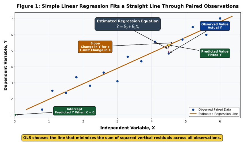
Figure 1 illustrates the main pieces of a simple linear regression. Each point is a paired observation of \(X\) and \(Y\). The fitted line represents the estimated relationship. The vertical distance from an observed point to the fitted line is the residual. A good regression line does not pass through every point. It balances the prediction errors across the sample according to the least squares criterion.

Example 1: Interpreting a Simple Linear Regression Equation

An analyst estimates the relationship between monthly excess returns on a listed clean‑energy fund and monthly excess returns on a broad equity market index. The estimated regression equation is:

$$ \hat{R}_{\text{Fund}} = 0.004 + 1.25R_{\text{Market}} $$

Interpret the intercept and slope in plain investment language.

Solution

Recall the estimated regression equation:

$$ \hat{Y}_i = \hat{b}_0 + \hat{b}_1 X_i $$

Where:

• \(\hat{Y}_i = \hat{R}_{\text{Fund}}\), the predicted monthly excess return on the fund
• \(X_i = R_{\text{Market}}\), the monthly excess return on the market index
• \(\hat{b}_0 = 0.004\), the estimated intercept
• \(\hat{b}_1 = 1.25\), the estimated slope coefficient

The intercept of 0.004 means that when the market excess return is 0.00%, the model predicts a fund excess return of 0.40%. This should not automatically be interpreted as skill. The analyst must still test whether the intercept is statistically significant and economically meaningful.

The slope of 1.25 means that for a one-unit increase in the market excess return, the fund’s predicted excess return increases by 1.25 units. If returns are expressed in decimal form, a one-percentage-point increase in the market excess return is associated with a 1.25-percentage-point increase in the fund’s predicted excess return.

If the market excess return is 3.0%, the predicted fund excess return is:

$$ \hat{R}_{\text{Fund}} = 0.004 + 1.25(0.030) = 0.0415 = 4.15\% $$

The fund has positive market sensitivity. The regression result suggests that it tends to amplify broad equity market movements.

Indicator Variables in Simple Regression

Simple regression can also use an indicator variable, sometimes called a dummy variable. An indicator variable takes the value 1 if a condition is true and 0 if it is not.

An indicator variable can be defined as:

$$ I(A) = \{1, \text{ if event } A \text{ occurs } 0, \text{ if event } A \text{ does not occur} $$

Where:

• \(I(A)\) is the indicator variable for event \(A\)
• \(A\) is the event or condition being evaluated
• 1 indicates that the event occurs
• 0 indicates that the event does not occur

When an indicator variable is used as the independent variable, the simple regression model becomes:

$$ Y_i = b_0 + b_1 I(A_i) + \epsilon_i $$

Where:

• \(Y_i\) is the dependent variable for observation \(i\)
• \(I(A_i)\) is the indicator variable for observation \(i\)
• \(b_0\) is the mean value of \(Y\) when the indicator equals 0
• \(b_1\) is the difference in the mean value of \(Y\) when the indicator changes from 0 to 1
• \(\epsilon_i\) is the error term

The intercept is the baseline mean. The slope is the estimated difference between the two groups.

Example 2: Using an Indicator Variable to Capture a Regime Shift

Assume we have monthly bank-stock excess returns before and after a major regulatory capital reform. The analyst defines an indicator variable, \(POST\), equal to 1 after the reform and 0 before the reform. The estimated regression equation is:

$$ \hat{R}_{\text{Bank}} = 0.006 – 0.004(\text{POST}) $$

Interpret the effect of the regulatory reform period on average excess returns.

Solution

Recall that:

$$ \hat{Y}_i = \hat{b}_0 + \hat{b}_1 I(A_i) $$

Where:

• \(\hat{Y}_i = \hat{R}_{\text{Bank}}\), the predicted monthly bank-stock excess return
• \(I(A_i) = POST\), the indicator variable equal to 1 after the reform and 0 before the reform
• \(\hat{b}_0 = 0.006\), the estimated average monthly excess return before the reform
• \(\hat{b}_1 = -0.004\), the estimated difference in average monthly excess return after the reform

Before the reform, \(POST = 0\):

$$\hat{R}_{\text{Bank}} = 0.006 – 0.004(0) = 0.006 = 0.60\%$$

After the reform, \(POST = 1\):

$$\hat{R}_{\text{Bank}} = 0.006 – 0.004(1) = 0.002 = 0.20\%$$

The estimated average monthly bank-stock excess return is 0.40 percentage points lower after the reform. The regression does not by itself prove that the reform caused the lower average return. It quantifies the difference associated with the indicator variable in the observed sample.

Residuals and Prediction Errors

The residual is the difference between the observed value and the fitted value:

$$e_i = Y_i – \hat{Y}_i$$

Where:

• \(e_i\) is the residual for observation \(i\)
• \(Y_i\) is the observed value of the dependent variable
• \(\hat{Y}_i\) is the predicted value from the estimated regression equation

A positive residual means that the observed Y is above the predicted value. A negative residual means that the observed \(Y\) is below the predicted value.

Residuals are estimates of model errors. They are not the same as the true error terms because the true regression line is unknown. Residuals come from the fitted model and are used to assess how well the line fits the data.

Figure 2: Residuals Show the Vertical Prediction Errors Around the Fitted Line

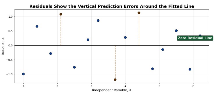
Figure 2 plots residuals against the independent variable. The horizontal line at zero represents perfect prediction. Points above the line are positive residuals, and points below the line are negative residuals. A random scatter around zero is usually more reassuring than a visible pattern. A pattern may suggest that the simple linear model is missing an important feature of the relationship.

Example 3: Calculating a Predicted Value and Residual

Let’s say an analyst estimates the following relationship between a company’s quarterly revenue growth and its quarterly operating margin:

$$\hat{\text{Margin}} = 0.055 + 0.70(\text{Revenue Growth})$$

Revenue growth and operating margin are both expressed in decimal form. In one quarter, revenue growth is 8.0%, and the actual operating margin is 12.4%.

Calculate the predicted operating margin and the residual.

Solution

We know that the predicted-value equation is given by:

$$\hat{Y}_i = \hat{b}_0 + \hat{b}_1 X_i$$

Where:

• \(\hat{Y}_i\) is the predicted operating margin
• \(\hat{b}_0 = 0.055\), the estimated intercept
• \(\hat{b}_1 = 0.70\), the estimated slope coefficient
• \(X_i = 0.080\), the quarterly revenue growth rate

The predicted operating margin is:

$$\hat{\text{Margin}} = 0.055 + 0.70(0.080) = 0.111 = 11.1\%$$

We know that:

$$e_i = Y_i – \hat{Y}_i$$

Where:

• \(Y_i = 12.4\%\), the observed operating margin
• \(\hat{Y}_i = 11.1\%\), the predicted operating margin

So that the residual is:

$$e_i = 12.4\% – 11.1\% = 1.3\%$$

The actual margin was 1.3 percentage points above the model’s prediction.

The Least Squares Criterion

Ordinary least squares, or OLS, chooses the intercept and slope that minimize the sum of squared residuals. The sum of squared residuals is also called the sum of squared errors, or SSE:

$$SSE = \sum_{i=1}^{n} e_i^2 = \sum_{i=1}^{n} \left(Y_i – \hat{Y}_i\right)^2 = \sum_{i=1}^{n} \left[Y_i – \left(\hat{b}_0 + \hat{b}_1 X_i\right)\right]^2$$

Where:

• \(SSE\) is the sum of squared errors
• \(e_i\) is the residual for observation \(i\)
• \(Y_i\) is the observed value of the dependent variable
• \(\hat{Y}_i\) is the predicted value from the regression equation
• \(\hat{b}_0\) is the estimated intercept
• \(\hat{b}_1\) is the estimated slope coefficient
• \(X_i\) is the observed value of the independent variable
• \(n\) is the number of observations

OLS squares the residuals before adding them. Squaring serves two purposes. First, positive and negative residuals do not cancel out. Second, large prediction errors receive more weight than small prediction errors. This is why OLS can be sensitive to outliers.

Example 4: Comparing Two Candidate Regression Lines Using SSE

Consider three observations for an analyst trying to explain active fund return, \(Y\), using benchmark return, \(X\):

$$
\begin{array}{c|c|c}
\textbf{Observation} & \textbf{X} & \textbf{Y} \\ \hline
1 & 1.0\% & 1.8\% \\ \hline
2 & 2.0\% & 2.6\% \\ \hline
3 & 3.0\% & 3.1\% \\
\end{array}
$$

Two candidate fitted lines are being compared:

$$\hat{Y} = 1.0\% + 0.70X$$

$$\hat{Y} = 0.5\% + 0.90X$$

Identify which candidate line fits better under the least squares criterion.

Solution

Start with the SSE formula:

$$SSE = \sum_{i=1}^{n} \left(Y_i – \hat{Y}_i\right)^2$$

Where:

• \(SSE\) is the sum of squared errors
• \(Y_i\) is the observed active fund return
• \(\hat{Y}_i\) is the predicted active fund return
• \(n = 3\), the number of observations

For Candidate Line 1:

$$\begin{array}{c|c|c|c|c}
\textbf{Observation} & \textbf{Y} & \textbf{Predicted Y} & \textbf{Residual} & \textbf{Squared Residual} \\ \hline
1 & 1.8\% & 1.7\% & 0.1\% & 0.000001 \\ \hline
2 & 2.6\% & 2.4\% & 0.2\% & 0.000004 \\ \hline
3 & 3.1\% & 3.1\% & 0.0\% & 0.000000 \\ \hline
\text{Total} & & & & 0.000005 \\
\end{array}$$

For Candidate Line 2:

$$\begin{array}{c|c|c|c|c}
\textbf{Observation} & \textbf{Y} & \textbf{Predicted Y} & \textbf{Residual} & \textbf{Squared Residual} \\ \hline
1 & 1.8\% & 1.4\% & 0.4\% & 0.000016 \\ \hline
2 & 2.6\% & 2.3\% & 0.3\% & 0.000009 \\ \hline
3 & 3.1\% & 3.2\% & -0.1\% & 0.000001 \\ \hline
\text{Total} & & & & 0.000026 \\
\end{array}$$

Candidate Line 1 has the lower SSE, so it fits better under the least squares criterion. OLS selects the line with the minimum possible SSE among all straight lines.

Estimating the Slope Coefficient

The OLS slope coefficient can be written as the ratio of the sample covariance between \(X\) and \(Y\) to the sample variance of \(X\):

$$\hat{b}_1 = \frac{s_{X,Y}}{s_X^2}$$

Where:

• \(\hat{b}_1\) is the estimated slope coefficient
• \(s_{X,Y}\) is the sample covariance between \(X\) and \(Y\)
• \(s_X^2\) is the sample variance of \(X\)

Equivalently, the slope can be calculated directly from deviations from the sample means:

$$\hat{b}_1 = \frac{\sum_{i=1}^{n} (X_i – \bar{X})(Y_i – \bar{Y})}{\sum_{i=1}^{n} (X_i – \bar{X})^2}$$

Where:

• \(\bar{X}\) is the sample mean of the independent variable
• \(\bar{Y}\) is the sample mean of the dependent variable
• \(X_i – \bar{X}\) is the deviation of observation \(i\) of \(X\) from its mean
• \(Y_i – \bar{Y}\) is the deviation of observation \(i\) of \(Y\) from its mean

This formula shows why the slope is tied to co-movement. If high values of \(X\) tend to appear with high values of \(Y\), the numerator is positive and the slope is positive. If high values of \(X\) tend to appear with low values of \(Y\), the numerator is negative and the slope is negative.

Estimating the Intercept

Once the slope has been estimated, the intercept is calculated using the sample means:

$$\hat{b}_0 = \bar{Y} – \hat{b}_1 \bar{X}$$

Where:

• \(\hat{b}_0\) is the estimated intercept
• \(\bar{Y}\) is the sample mean of the dependent variable
• \(\hat{b}_1\) is the estimated slope coefficient
• \(\bar{X}\) is the sample mean of the independent variable

This formula implies an important OLS property: the fitted regression line passes through the point \((\bar{X}, \bar{Y})\). In plain language, when \(X\) is at its sample mean, the predicted value of \(Y\) equals the sample mean of \(Y\).

Another important OLS property is:

$$\sum_{i=1}^{n} e_i = 0$$

Where:

• \(e_i\) is the residual for observation \(i\)
• \(n\) is the number of observations

The residuals sum to zero when the regression includes an intercept. This property helps explain why OLS balances positive and negative prediction errors around the fitted line.

Example 5: Estimating the Slope and Intercept

Assume we are estimating a simple regression of monthly subscription revenue growth, \(Y\), on monthly marketing-spend growth, \(X\), for a financial technology company. The paired observations are:

$$ \begin{array}{c|c|c}
\textbf{Month} & \textbf{Marketing-Spend Growth, X} & \textbf{Revenue Growth, Y} \\ \hline
1 & 1.0\% & 2.0\% \\ \hline
2 & 2.0\% & 2.7\% \\ \hline
3 & 4.0\% & 4.0\% \\ \hline
4 & 5.0\% & 4.9\% \\
\end{array}
$$

Estimate the slope, intercept, and fitted regression equation.

Solution

We know that:

$$\hat{b}_1 = \frac{\sum_{i=1}^{n} (X_i – \bar{X})(Y_i – \bar{Y})}{\sum_{i=1}^{n} (X_i – \bar{X})^2}$$

Where:

• \(\hat{b}_1\) is the estimated slope coefficient
• \(X_i\) is marketing-spend growth in month \(i\)
• \(Y_i\) is subscription revenue growth in month \(i\)
• \(\bar{X}\) is the sample mean of marketing-spend growth
• \(\bar{Y}\) is the sample mean of subscription revenue growth
• \(n = 4\), the number of monthly observations

First, calculate the sample means:

$$\bar{X} = \frac{1.0\% + 2.0\% + 4.0\% + 5.0\%}{4} = 3.0\%$$

$$\bar{Y} = \frac{2.0\% + 2.7\% + 4.0\% + 4.9\%}{4} = 3.4\%$$

Now calculate deviations and products:

$$\begin{array}{c|c|c|c|c}
\textbf{Month} & X_i – \bar{X} & Y_i – \bar{Y} & \textbf{Product} & (X_i – \bar{X})^2 \\ \hline
1 & -2.0\% & -1.4\% & 0.00028 & 0.00040 \\ \hline
2 & -1.0\% & -0.7\% & 0.00007 & 0.00010 \\ \hline
3 & 1.0\% & 0.6\% & 0.00006 & 0.00010 \\ \hline
4 & 2.0\% & 1.5\% & 0.00030 & 0.00040 \\ \hline
\text{Total} & & & 0.00071 & 0.00100 \\
\end{array}$$

The slope is:

$$\hat{b}_1 = \frac{0.00071}{0.00100} = 0.71$$

Now, using the intercept formula:

$$\hat{b}_0 = \bar{Y} – \hat{b}_1 \bar{X}$$

Where:

• \(\hat{b}_0\) is the estimated intercept
• \(\bar{Y} = 3.4\%\) is the sample mean revenue growth
• \(\hat{b}_1 = 0.71\) is the estimated slope
• \(\bar{X} = 3.0\%\) is the sample mean marketing-spend growth

The intercept is therefore:

$$\hat{b}_0 = 0.034 – 0.71(0.030) = 0.0127 = 1.27\%$$

Consequently, the fitted regression equation is:

$$\hat{Y} = 1.27\% + 0.71X$$

The slope indicates that a one-percentage-point increase in marketing-spend growth is associated with a 0.71-percentage-point increase in predicted subscription revenue growth. The intercept indicates predicted revenue growth of 1.27% when marketing-spend growth is zero, within the context of this sample and model.

Cross-Sectional, Time-Series, and Panel Data

Regression can be applied to different data structures. The structure affects interpretation and the types of problems the analyst must watch for.

Figure 3: Regression Data Structures

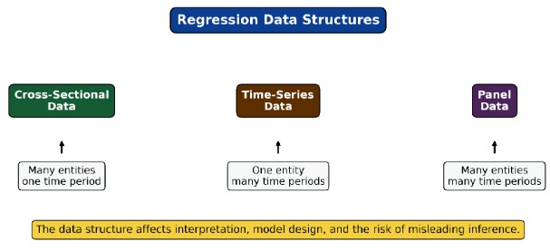
Figure 3 separates the main data structures used in regression. Cross-sectional data compare many entities at a single point in time. Time-series data follow one entity or variable across time. Panel data combine both dimensions by tracking many entities across multiple periods. A regression on stock returns over time is not interpreted in the same way as a regression comparing valuation multiples across companies at a date.

$$ \textbf{Table 2: Types of Data Used in Regression} \\
\begin{array}{l|l|l|l}
\textbf{Data Type} & \textbf{Basic Structure} & \textbf{Finance Example} & \textbf{Key Interpretation Issue} \\ \hline
\text{Cross-sectional data} & \text{Many entities at one point} & \text{Revenue growth and} & \text{Differences across} \\
& \text{in time} & \text{valuation multiples across} & \text{entities may reflect} \\
& & \text{80 companies in the} & \text{omitted characteristics} \\
& & \text{same quarter} & \\ \hline
\text{Time-series data} & \text{One entity across many} & \text{Monthly portfolio return} & \text{Relationships may} \\
& \text{periods} & \text{and monthly market} & \text{change across regimes} \\
& & \text{return over five years} & \\ \hline
\text{Panel data} & \text{Many entities across} & \text{Quarterly margins and} & \text{Both entity-specific and} \\
& \text{many periods} & \text{sales growth for 40} & \text{time-specific effects may} \\
& & \text{companies over 10 years} & \text{matter} \\
\end{array}
$$

Table 2 summarizes the practical distinction. Cross-sectional analysis emphasizes differences across entities. Time-series analysis emphasizes variation over time. Panel analysis can examine both, but it is also more complex.

Correlation, Regression, and Causation

Regression uses statistical association to estimate relationships. A strong slope or visible pattern does not prove causation. This is especially important in finance, where variables may move together because of a common driver.

For example, a positive relationship between technology-stock returns and semiconductor demand may reflect a real economic link, but it may also reflect broader risk appetite, interest-rate expectations, or common exposure to growth-style equities. Regression can quantify the relationship in the data. It cannot by itself prove the causal mechanism.

The analyst should therefore ask three questions:

• Is the relationship statistically supported?
• Is the relationship economically plausible?
• Could another variable or regime change explain the result?

The last question is especially important. Financial relationships can break down when policy regimes, inflation environments, liquidity conditions, or investor positioning changes.

Interpretation and Evaluation

Several practical principles follow:

• Simple linear regression models one dependent variable using one independent variable.
• The slope measures the expected change in the dependent variable for a one-unit change in the independent variable.
• The intercept is the fitted value of the dependent variable when the independent variable is zero.
• The residual is the observed value minus the predicted value.
• OLS chooses the line that minimizes the sum of squared residuals.
• The OLS slope can be expressed as the covariance between \(X\) and \(Y\) divided by the variance of \(X\).
• The OLS intercept is calculated from the sample means after the slope is estimated.
• With an intercept, the OLS line passes through \((\bar{X}, \bar{Y})\) and residuals sum to zero.
• Indicator variables allow regression to estimate differences between groups or regimes.
• Regression identifies association, not causation, unless the research design supports a causal claim.

Question

An analyst estimates the following regression using monthly data:

$$\hat{R}_{\text{Portfolio}} = 0.002 + 0.85R_{\text{Factor}}$$

Both returns are expressed in decimal form. In a month when the factor return is 4.0%, the portfolio’s actual return is 3.2%. The residual for that month is closest to:

1. -0.40%
2. 0.00%
3. 0.40%

Answer Explanation

The correct answer is A.

Start by quoting the predicted-value equation:

$$\hat{Y}_i = \hat{b}_0 + \hat{b}_1 X_i$$

Where:

• \(\hat{Y}_i\) is the predicted monthly portfolio return
• \(\hat{b}_0 = 0.002\), the estimated intercept
• \(\hat{b}_1 = 0.85\), the estimated slope coefficient
• \(X_i = 0.040\), the monthly factor return

The predicted portfolio return is:

$$\hat{R}_{\text{Portfolio}} = 0.002 + 0.85(0.040) = 0.036 = 3.60\%$$

Now quote the residual formula:

$$e_i = Y_i – \hat{Y}_i$$

Where:

• \(e_i\) is the residual for the month
• \(Y_i = 3.20\%\), the observed portfolio return
• \(\hat{Y}_i = 3.60\%\), the predicted portfolio return

The residual is:

$$e_i = 3.20\% – 3.60\% = -0.40\%$$

The residual is -0.40%, meaning the portfolio return was 0.40 percentage points below the model’s prediction.

B is incorrect because it would be the residual only if the actual return equaled the predicted return.

C is incorrect because it reverses the residual sign by subtracting the actual value from the predicted value rather than subtracting the predicted value from the actual value.