Regression Assumptions, Residual Analysis, Goodness of Fit, Coefficients, and ANOVA in Finance

The first step in regression is estimating a line. The second, more important step is deciding whether the estimated line deserves the analyst’s confidence. A regression output can look mathematically precise while still being economically misleading. The slope can be significant for the wrong reason. A high \(R^2\) can hide a poor model. A clean-looking equation can be damaged by nonlinearity, heteroskedasticity, autocorrelation, or non-normal residuals.

This learning outcome focuses on the discipline required after the regression is estimated. The analyst must understand the assumptions behind simple linear regression, use residual analysis to identify possible violations, evaluate goodness-of-fit, interpret coefficient tests, and read the analysis of variance, or ANOVA, output.

The practical question is not simply, “What is the regression line?” The better question is, “Is this line a reliable way to explain the relationship between the variables?”

Review of the Simple Linear Regression Model

The simple linear regression model is:

$$Y_i = b_0 + b_1 X_i + \epsilon_i$$

Where:

• \(Y_i\) is the observed value of the dependent variable for observation \(i\)
• \(X_i\) is the observed value of the independent variable for observation \(i\)
• \(b_0\) is the population intercept
• \(b_1\) is the population slope coefficient
• \(\epsilon_i\) is the error term for observation \(i\)

The estimated regression equation is:

$$\hat{Y}_i = \hat{b}_0 + \hat{b}_1 X_i$$

Where:

• \(\hat{Y}_i\) is the predicted value of the dependent variable
• \(\hat{b}_0\) is the estimated intercept
• \(\hat{b}_1\) is the estimated slope coefficient
• \(X_i\) is the observed independent variable

The residual is:

$$e_i = Y_i – \hat{Y}_i$$

Where:

• \(e_i\) is the residual for observation \(i\)
• \(Y_i\) is the observed value of the dependent variable
• \(\hat{Y}_i\) is the predicted value from the estimated regression equation

The residual is the observable diagnostic tool. The true error term, \(\epsilon_i\), is unobservable, but residuals help the analyst infer whether the model is likely to be misspecified.

Main Assumptions of Simple Linear Regression

Simple linear regression relies on assumptions about the relationship between the variables and the behavior of the error terms. These assumptions make inference meaningful. If they fail, the fitted line may still minimize squared residuals, but coefficient tests, p-values, prediction intervals, and conclusions may become unreliable.

Figure 1: Four Core Assumptions of Simple Linear Regression

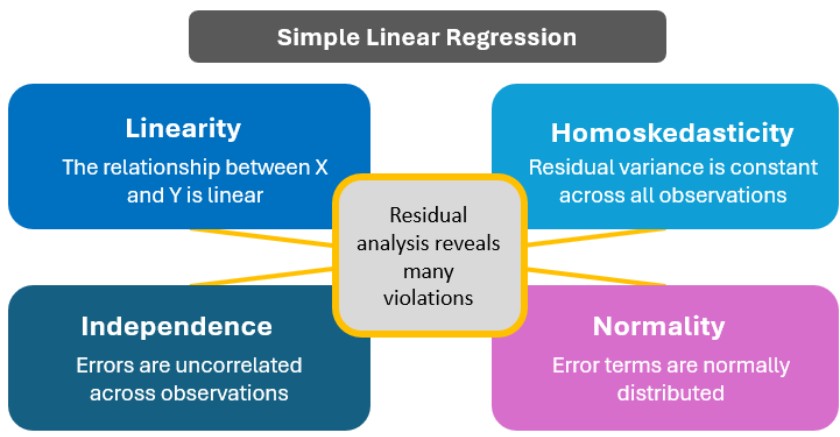
Figure 1 summarizes the four central assumptions: linearity, homoskedasticity, independence, and normality. In practice, the analyst often begins by examining residuals. Clean residuals do not prove the model is perfect, but patterned residuals are a warning sign that the model may be missing an important feature of the data.

$$ \textbf{Table 1: Regression Assumptions, Violations, and Diagnostic Clues} \\
\begin{array}{l|l|l|l|l}
\textbf{Assumption} & \textbf{Meaning} & \textbf{Typical Violation} & \textbf{Residual Clue} & \textbf{Main Concern} \\ \hline
\text{Linearity} & \text{The expected value} & \text{True relationship is} & \text{U-shape or} & \text{Biased fitted values} \\
& \text{of } Y \text{ is a linear} & \text{curved} & \text{systematic pattern} & \text{in parts of the data} \\
& \text{function of } X & & & \text{range} \\ \hline
\text{Homoskedasticity} & \text{Error variance is} & \text{Error variance} & \text{Funnel shape or} & \text{Standard errors and} \\
& \text{constant across} & \text{changes with } X \text{ or} & \text{regime-dependent} & \text{tests may be} \\
& \text{observations} & \text{across groups} & \text{spread} & \text{unreliable} \\ \hline
\text{Independence} & \text{Error terms are} & \text{Autocorrelation or} & \text{Runs, waves, or} & \text{Coefficient} \\
& \text{uncorrelated across} & \text{serial correlation} & \text{cycles in residuals} & \text{inference may be} \\
& \text{observations} & & & \text{invalid} \\ \hline
\text{Normality} & \text{Error terms are} & \text{Skewed or fat-tailed} & \text{Skewed histogram} & \text{Small-sample} \\
& \text{normally distributed} & \text{errors} & \text{or extreme} & \text{hypothesis tests} \\
& & & \text{residuals} & \text{may be unreliable} \\ \hline
\end{array}
$$

Table 1 is useful because each assumption has a different diagnostic signature. A U-shaped residual plot points toward a nonlinearity problem. A funnel-shaped plot points toward heteroskedasticity. A cyclical residual pattern points toward autocorrelation. A skewed residual histogram points toward non-normality.

Assumption 1: Linearity

The linearity assumption means that the dependent variable is related to the independent variable in a straight-line form:

$$E(Y_i | X_i) = b_0 + b_1 X_i$$

Where:

• \(E(Y_i | X_i)\) is the expected value of \(Y_i\) conditional on \(X_i\)
• \(b_0\) is the intercept
• \(b_1\) is the slope coefficient
• \(X_i\) is the independent variable

If the true relationship is curved, a straight-line model can systematically overpredict some observations and underpredict others. This may show up as a pattern in the residuals.

Example 1: Recognizing a Linearity Violation

Imagine a credit analyst regresses loan default rates on borrower debt-to-income ratios. At low debt-to-income levels, default rates increase slowly. At high debt-to-income levels, default rates rise sharply. A straight line is fitted anyway.

If the residuals are negative at low \(X\), positive in the middle, and negative again at high \(X\), the residual plot may show a U-shaped or inverted-U-shaped pattern. That pattern suggests the linearity assumption is violated. The model may need a transformed variable, a nonlinear term, or a different specification.

The key exam point is that ordinary least squares still produces a line. The problem is not that the line cannot be estimated. The problem is that the line may be the wrong shape for the relationship.

Assumption 2: Homoskedasticity

Homoskedasticity means that the variance of the error terms is constant across observations:

$$E\left(\epsilon_i^2\right) = \sigma_{\epsilon}^2, \quad i = 1, 2, \dots, n$$

Where:

• \(E\left(\epsilon_i^2\right)\) is the expected squared error term for observation \(i\)
• \(\sigma_{\epsilon}^2\) is the constant error variance
• \(n\) is the number of observations

If the variance of the error terms differs across observations, the regression has heteroskedasticity. This is common in financial data. Large firms may have lower return volatility than small firms. Stress periods may have much larger residuals than calm periods. High-yield bonds may show greater unexplained spread changes than investment-grade bonds.

Heteroskedasticity often appears as a funnel shape in a residual plot. The residuals may be tightly clustered for low values of \(X\) and widely dispersed for high values of \(X\), or vice versa.

Example 2: Diagnosing Heteroskedasticity in Equity Returns

Assume we have a regression of weekly individual stock returns on weekly market returns across a sample that includes both mega-cap and micro-cap companies. The residuals for mega-cap stocks cluster narrowly around zero, while residuals for micro-cap stocks spread widely.

This is a classic warning sign. The variance of the residuals is not constant across the sample. The model may still estimate a slope, but the usual standard errors may be unreliable. A candidate should identify this as a homoskedasticity violation, not as a linearity violation.

Assumption 3: Independence

The independence assumption means that error terms are uncorrelated across observations. In practical terms, one residual should not help predict the next residual.

Autocorrelation is a common violation in time-series data. If positive residuals tend to be followed by positive residuals, and negative residuals tend to be followed by negative residuals, the errors are not independent. This can happen when an omitted variable moves slowly over time, when markets trend, or when the dependent variable adjusts gradually.

Example 3: Identifying Autocorrelation from Residuals

Let’s say an analyst regresses monthly fund flows on prior-month performance. The residual plot is ordered by month. For several months, residuals are mostly positive; for the next several months, residuals are mostly negative; later, they become positive again.

That wave-like behavior suggests autocorrelation. The residuals are not randomly scattered across time. This undermines the independence assumption and may make the regression’s inference too optimistic.

Assumption 4: Normality

The normality assumption requires the error terms to be normally distributed. This assumption matters most for small-sample hypothesis tests. It does not require the dependent variable or independent variable to be normally distributed. The focus is on the error terms.

Because true error terms are unobservable, analysts inspect residuals. A roughly bell-shaped residual histogram supports the normality assumption. A strongly skewed histogram, heavy tails, or extreme residuals may signal a violation.

For large samples, the central limit theorem can reduce the practical importance of exact normality for inference. Still, in CFA-style questions, candidates must know that normality applies to the error terms, not necessarily to \(X\) or \(Y\).

Residual Analysis as a Diagnostic Tool

Residual analysis is the bridge between model estimation and model evaluation. It helps identify whether the model’s assumptions look reasonable.

Figure 2: Residual Plots Help Detect Regression Assumption Violations

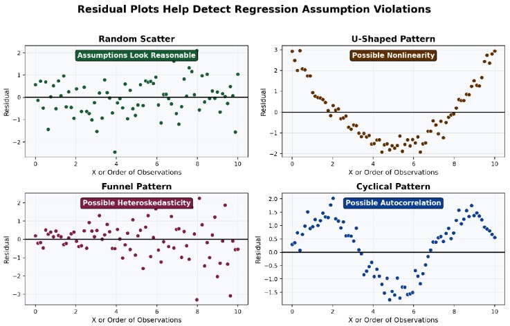
Figure 2 compares four residual patterns. Random scatter around zero is usually consistent with a well-specified linear model. A U-shaped pattern suggests nonlinearity. A funnel pattern suggests heteroskedasticity. A cyclical pattern suggests autocorrelation. The important exam skill is matching the residual pattern to the violated assumption.

A strong candidate should not overclaim. A residual plot indicates a possible issue; it is not a formal proof. It tells the analyst what to investigate next.

Total, Explained, and Unexplained Variation

Goodness-of-fit begins with variation in the dependent variable. Regression decomposes total variation into explained and unexplained components.

The total sum of squares is:

$$SST = \sum_{i=1}^{n} \left(Y_i – \bar{Y}\right)^2$$

Where:

• \(SST\) is the total sum of squares
• \(Y_i\) is the observed value of the dependent variable
• \(\bar{Y}\) is the sample mean of the dependent variable
• \(n\) is the number of observations

The regression sum of squares is:

$$SSR = \sum_{i=1}^{n} \left(\hat{Y}_i – \bar{Y}\right)^2$$

Where:

• \(SSR\) is the regression sum of squares
• \(\hat{Y}_i\) is the predicted value from the regression equation
• \(\bar{Y}\) is the sample mean of the dependent variable

The sum of squared errors is:

$$SSE = \sum_{i=1}^{n} \left(Y_i – \hat{Y}_i\right)^2$$

Where:

• \(SSE\) is the sum of squared errors
• \(Y_i\) is the observed value of the dependent variable
• \(\hat{Y}_i\) is the predicted value from the reg

The relationship among these components is:

$$SST = SSR + SSE$$

Where:

• \(SST\) is total variation
• \(SSR\) is variation explained by the regression
• \(SSE\) is unexplained residual variation

Figure 3: ANOVA Decomposition of Total Variation

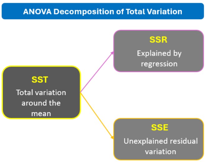
Figure 3 shows the logic behind regression ANOVA. Total variation in the dependent variable is split into explained variation and unexplained variation. The higher the explained share, the better the model describes variation in the sample. However, fit is not the same as validity. A model can have a high \(R^2\) and still violate assumptions or lack economic meaning.

Coefficient of Determination

The coefficient of determination, or \(R^2\), measures the proportion of total variation in the dependent variable explained by the regression:

$$R^2 = \frac{SSR}{SST}$$

Where:

• \(R^2\) is the coefficient of determination
• \(SSR\) is the regression sum of squares
• \(SST\) is the total sum of squares

Because \(SST = SSR + SSE\), \(R^2\) can also be understood as the explained share of total variation. If \(R^2 = 0.72\), the model explains 72% of the variation in \(Y\) within the sample.

In simple linear regression, \(R^2\) is the square of the sample correlation between \(X\) and \(Y\):

$$R^2 = r^2$$

Where:

• \(r\) is the sample correlation between \(X\) and \(Y\)
• \(R^2\) is the coefficient of determination

This relationship holds in simple linear regression with one independent variable. It should not be casually extended to more complex settings without care.

Example 4: Calculating \(R^2\) from Sum of Squares

Consider a regression of monthly luxury-retail stock returns on monthly consumer-confidence changes. The model produces the following sums of squares:

$$\begin{array}{l|l}
\textbf{Component} & \textbf{Value} \\ \hline
\text{Sum of squares regression, } SSR & 0.0245 \\ \hline
\text{Sum of squared errors, } SSE & 0.0105 \\
\end{array}$$

Calculate the coefficient of determination.

Solution

Recall that:

$$SST = SSR + SSE$$

Where:

• \(SST\) is total variation in monthly stock returns
• \(SSR = 0.0245\) is explained variation
• \(SSE = 0.0105\) is unexplained variation

Calculate total variation:

$$SST = 0.0245 + 0.0105 = 0.0350$$

Now quote the \(R^2\) formula:

$$R^2 = \frac{SSR}{SST}$$

Where:

• \(R^2\) is the proportion of total variation explained by the regression
• \(SSR = 0.0245\) is explained variation
• \(SST = 0.0350\) is total variation

Calculate:

$$R^2 = \frac{0.0245}{0.0350} = 0.7000 = 70.0\%$$

The regression explains 70.0% of the sample variation in monthly luxury-retail stock returns. The remaining 30.0% is unexplained by the model.

Standard Error of the Estimate

The standard error of the estimate, also called the standard error of the regression, measures the typical distance between observed values and fitted values. It is calculated as the square root of mean squared error:

$$s_e = \sqrt{MSE}$$

Where:

• \(s_e\) is the standard error of the estimate
• \(MSE\) is the mean squared error

For simple linear regression:

$$MSE = \frac{SSE}{n-2}$$

Where:

• \(MSE\) is the mean squared error
• \(SSE\) is the sum of squared errors
• \(n – 2\) is the degrees of freedom for error in simple linear regression

Combining the two formulas:

$$s_e = \sqrt{\frac{SSE}{n-2}}$$

Where:

• \(s_e\) is the standard error of the estimate
• \(SSE\) is the sum of squared errors
• \(n\) is the sample size

A smaller standard error of the estimate indicates that observed values tend to be closer to the fitted regression line. Unlike \(R^2\), which is a relative fit measure, \(s_e\) is in the units of the dependent variable.

ANOVA Table and the F-Statistic

An ANOVA table organizes regression variation into regression, error, and total components. For simple linear regression, the typical structure is:

$$ \textbf{Table 2: ANOVA Table for Simple Linear Regression} \\
\begin{array}{l|c|c|c|c}
\textbf{Source} & \textbf{Sum of Squares} & \textbf{Degrees of Freedom} & \textbf{Mean Square} & \textbf{F-Statistic} \\
\hline
\text{Regression} & SSR & 1 & MSR = \frac{SSR}{1} & F = MSR/MSE \\ \hline
\text{Error} & SSE & n – 2 & MSE =\frac {SSE}{(n – 2)} & \\ \hline
\text{Total} & SST & n – 1 & & \\
\end{array}
$$

Table 2 shows how the F-statistic is constructed. Mean square regression measures explained variation per regression degree of freedom. Mean square error measures unexplained variation per error degree of freedom. The F-statistic compares the two.

The mean square regression is:

$$MSR = \frac{SSR}{k}$$

Where:

• \(MSR\) is the mean square regression
• \(SSR\) is the regression sum of squares
• \(k\) is the number of independent variables

For simple linear regression, \(k = 1\), so \(MSR = SSR\).

The F-statistic is:

$$F = \frac{MSR}{MSE}$$

Where:

• \(F\) is the F-statistic
• \(MSR\) is the mean square regression
• \(MSE\) is the mean squared error

A large F-statistic provides evidence against the null hypothesis that the slope coefficient is zero. In simple linear regression, the F-test of the overall model and the t-test of the slope coefficient have the same significance conclusion.

Example 5: Reading an ANOVA Table

Assume an analyst estimates a regression of monthly infrastructure-fund excess returns on monthly inflation-surprise data using 28 observations. The results include:

$$
\begin{array}{l|c|c}
\textbf{Source} & \textbf{Sum of Squares} & \textbf{Degrees of Freedom} \\
\hline
\text{Regression} & 0.0180 & 1 \\ \hline
\text{Error} & 0.0091 & 26 \\ \hline
\text{Total} & 0.0271 & 27 \\
\end{array}
$$

Calculate \(R^2\), the standard error of the estimate, and the F-statistic.

Solution

Start with \(R^2\):

$$R^2 = \frac{SSR}{SST}$$

Where:

• \(SSR = 0.0180\) is explained variation
• \(SST = 0.0271\) is total variation

Calculate:

$$R^2 = \frac{0.0180}{0.0271} = 0.6642 = 66.42\%$$

Now we start with the standard error formula:

$$S_e = \sqrt{\frac{SSE}{n-2}}$$

Where:

• \(S_e\) is the standard error of the estimate
• \(SSE = 0.0091\) is unexplained variation
• \(n – 2 = 26\) is the error degrees of freedom

Calculate:

$$S_e = \sqrt{\frac{0.0091}{26}} = \sqrt{0.00035} = 0.0187$$

The typical prediction error is about 1.87 percentage points if returns are expressed in decimal form.

Now calculate the F-statistic:

$$F = \frac{MSR}{MSE}$$

Where:

• \(MSR = \frac {0.0180 }{ 1 }= 0.0180\) is the mean square regression
• \(MSE = \frac {0.0091 }{ 26} = 0.00035\) is mean squared error

Therefore:

$$F = \frac{0.0180}{0.00035} = 51.43$$

The F-statistic is large, suggesting that the regression explains a substantial amount of variation relative to residual variation. The analyst would still need the relevant p-value or critical value to make a formal hypothesis-test decision.

Testing Regression Coefficients

Regression analysis often tests whether a coefficient differs from a hypothesized value. For a slope coefficient, the hypotheses are commonly:

$$H_0 : b_1 = B_1$$

$$H_a : b_1 \neq B_1$$

Where:

• \(H_0\) is the null hypothesis
• \(H_a\) is the alternative hypothesis
• \(b_1\) is the population slope coefficient
• \(B_1\) is the hypothesized value of the slope coefficient

The t-statistic is:

$$t = \frac{\hat{b}_1 – B_1}{s_{\hat{b}_1}}$$

Where:

• \(t\) is the test statistic
• \(\hat{b}_1\) is the estimated slope coefficient
• \(B_1\) is the hypothesized slope coefficient under the null hypothesis
• \(s_{\hat{b}_1}\) is the standard error of the estimated slope coefficient

The t-statistic follows a t-distribution with \(n – 2\) degrees of freedom in simple linear regression. The analyst rejects the null hypothesis if the test statistic is sufficiently extreme or if the p-value is below the chosen significance level.

The intercept can be tested similarly:

$$t = \frac{\hat{b}_0 – B_0}{s_{\hat{b}_0}}$$

Where:

• \(\hat{b}_0\) is the estimated intercept
• \(B_0\) is the hypothesized intercept under the null hypothesis
• \(s_{\hat{b}_0}\) is the standard error of the estimated intercept

Example 6: Testing a Slope Coefficient

Suppose that a portfolio analyst regresses a factor fund’s monthly excess return on a quality-factor return. The estimated slope is 0.64, and the standard error of the slope is 0.18. Test whether the slope is different from zero at the 5% significance level.

Solution

Start by writing the hypotheses:

$$H_0 : b_1 = 0$$

$$H_a : b_1 \neq 0$$

We know that:

$$t = \frac{\hat{b}_1 – B_1}{s_{\hat{b}_1}}$$

Where:

• \(\hat{b}_1 = 0.64\) is the estimated slope coefficient
• \(B_1 = 0\) is the hypothesized slope coefficient
• \(s_{\hat{b}_1} = 0.18\) is the standard error of the slope estimate

Calculate:

$$t = \frac{0.64 – 0}{0.18} = 3.56$$

The calculated t-statistic is 3.56. For a two-sided 5% test, this is likely to be large enough to reject the null hypothesis in typical sample sizes. The analyst concludes that the slope is statistically different from zero, assuming the regression assumptions are sufficiently reliable.

p-Values and Statistical Significance

A p-value is the smallest level of significance at which the null hypothesis can be rejected. In regression output, p-values are often reported for the intercept, slope, and sometimes the F-statistic.

If the p-value is less than the significance level, reject the null hypothesis. If the p-value is greater than the significance level, fail to reject the null hypothesis.

$$ \textbf{Table 3: Interpreting p-Values in Regression Output} \\
\begin{array}{l|l|l}
{\textbf{p-Value Compared} \\ \textbf{with Significance} \\ \textbf{Level}} & \textbf{Decision} & \textbf{Interpretation} \\
\hline
\text{p-value } < \alpha & \text{Reject } H_0 & \text{Evidence is strong enough against the null hypothesis} \\ \hline \text{p-value } > \alpha & \text{Fail to reject } H_0 & \text{Evidence is not strong enough against the null hypothesis} \\ \hline
\text{p-value } = \alpha & \text{Borderline case} & \text{Follow the exam convention or stated decision rule}
\end{array}
$$

A smaller p-value does not prove that the relationship is economically important. It says that the observed result is unlikely under the null hypothesis, assuming the model and assumptions are valid. Economic significance must be evaluated separately.

Comparing Goodness-of-Fit Measures

$$ \textbf{Table 4: Goodness-of-Fit and Regression Output Metrics} \\
\begin{array}{l|l|l|l}
\textbf{Measure} & \textbf{Formula or Source} & \textbf{What It Answers} & \textbf{Better When} \\
\hline
R^2 & {\frac{SSR}{SST}} & {\text{What share of variation in}\\ Y \text{ is explained?}} & \text{Higher, subject to model validity} \\ \hline
\text{Standard error of the estimate} & \sqrt{\frac {SSE}{(n – 2)}} & {\text{How far are observed values from} \\ \text{fitted values on average?}} & \text{Lower} \\ \hline
\text{F-statistic} & {\frac{MSR}{MSE}} & {\text{Is explained variation large} \\ \text{relative to unexplained variation?}} & \text{Higher, for rejecting the null} \\ \hline
\text{t-statistic} & \frac {(\hat{b} – B)}{s_{\hat{b}}} & {\text{Is a coefficient different from} \\ \text{a hypothesized value?}} & \text{More extreme} \\ \hline
\text{p-value} & {\text{Reported in output or} \\ \text{derived from test statistic}} & \text{Is the result statistically significant at } \alpha\text{?} & \text{Lower}
\end{array}
$$

Table 4 is useful in interpretation questions. A high \(R^2\) describes fit. A low p-value supports statistical significance. A low standard error of the estimate indicates smaller prediction errors in the units of \(Y\). These are related but not interchangeable.

Interpretation and Evaluation

A strong regression interpretation goes beyond calculating output values. It connects the statistical result with the model assumptions and the investment problem.

Several practical principles follow:

• The dependent variable does not need to be normally distributed; the normality assumption applies to the error terms.
• A linearity violation often appears as a systematic residual pattern.
• Heteroskedasticity appears when residual variance changes across observations.
• Autocorrelation appears when residuals are correlated across observations, especially in time series.
• \(R^2\) measures the proportion of total variation in \(Y\) explained by the regression.
• The standard error of the estimate is an absolute measure of fit in the units of \(Y\).
• The ANOVA table decomposes total variation into explained and unexplained variation.
• In simple linear regression, the F-test for overall model significance and the t-test for the slope lead to the same significance conclusion.
• A statistically significant coefficient is not automatically economically meaningful.
• Residual analysis should complement, not replace, economic reasoning.

Question

An analyst estimates a simple linear regression using 42 monthly observations. The sum of squares regression is 0.084, and the sum of squared errors is 0.056. The standard error of the estimate and the coefficient of determination are closest to:

1. 0.0014 and 40.0%
2. 0.0374 and 60.0%
3. 0.0374 and 150.0%

Solution

The correct answer is B.

Recall the standard error of the estimate formula:

$$S_e = \sqrt{\frac{SSE}{n-2}}$$

Where:

• \(s_e\) is the standard error of the estimate
• \(SSE = 0.056\) is the sum of squared errors
• \(n = 42\) is the number of observations
• \(n – 2 = 40\) is the error degrees of freedom in simple linear regression

Calculate:

$$S_e = \sqrt{\frac{0.056}{40}} = \sqrt{0.0014} = 0.0374$$

Now calculate \(R^2\). First quote the total variation relationship:

$$SST = SSR + SSE$$

Where:

• \(SST\) is the total sum of squares
• \(SSR = 0.084\) is the regression sum of squares
• \(SSE = 0.056\) is the sum of squared errors

Therefore:

$$SST = 0.084 + 0.056 = 0.140$$

Now quote the coefficient of determination formula:

$$R^2 = \frac{SSR}{SST}$$

Where:

• \(R^2\) is the coefficient of determination
• \(SSR = 0.084\) is explained variation
• \(SST = 0.140\) is total variation

Calculate:

$$R^2 = \frac{0.084}{0.140} = 0.600 = 60.0\%$$

The standard error of the estimate is 0.0374, and the coefficient of determination is 60.0%.

A is incorrect because it uses the mean squared error, 0.0014, rather than taking the square root to calculate the standard error of the estimate. It also uses the unexplained portion, \(\frac {SSE}{SST}\), rather than the explained portion, \(\frac {SSR}{SST}\).

C is incorrect because the standard error is correct, but the \(R^2\) value is impossible. It incorrectly divides \(SSR\) by \(SSE\), producing \(\frac{0.084}{0.056} = 1.50\), or 150.0%.