Portfolio Return and Risk: Expected Return, Variance, Standard Deviation, Covariance, and Correlation

Portfolio Statistics Matter

A portfolio is more than a list of securities. Each security contributes return, but each also contributes risk and interacts with the other holdings. A high-volatility asset may increase portfolio risk sharply if it moves with the rest of the portfolio. The same asset may be much less dangerous if its returns are weakly correlated or negatively correlated with the other holdings.

This learning outcome brings together the main tools used to summarize portfolio return and risk. Expected return is a weighted average of the asset expected returns. Portfolio variance and standard deviation measure dispersion around expected return. Covariance and correlation show how asset returns move together. The central lesson is that portfolio risk depends not only on individual asset risk but also on co-movement.

These calculations are used every day in portfolio construction, risk reporting, manager evaluation, and strategic asset allocation. They also sit at the foundation of modern portfolio theory.

Figure 1: Portfolio Statistics Connect Return, Risk, and Co-Movement

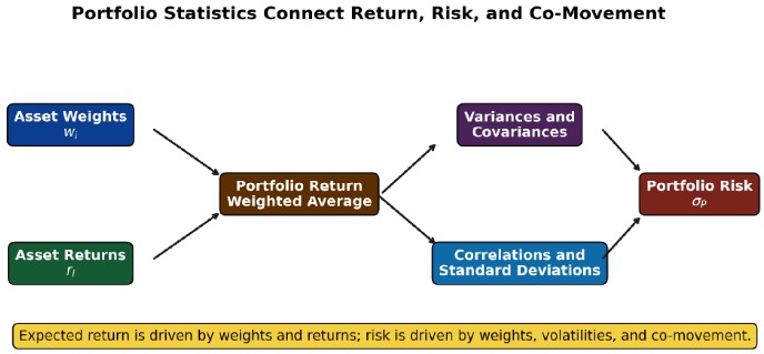
Figure 1 summarizes the logic of the learning outcome. Portfolio return starts with asset weights and asset returns. Portfolio risk requires more information: variances, standard deviations, covariances, and correlations. The important insight is that two portfolios with the same asset-level volatilities can have different portfolio standard deviations if the assets have different correlations.

Historical Portfolio Return

A historical portfolio return for a single period is the weighted average of the realized returns on the assets in the portfolio. The weights should normally be the weights at the beginning of the measurement period, because those weights determine how much capital was exposed to each asset during the period.

The one-period portfolio return is:

$$
r_{P,t} = \sum_{i=1}^{N} w_{i,t-1} r_{i,t}
$$

Where:

• \( r_{P,t} \) is the portfolio return in period \( t \)
• \( N \) is the number of assets in the portfolio
• \( w_{i,t-1} \) is the weight of asset \( i \) at the beginning of period \( t \)
• \( r_{i,t} \) is the realized return of asset \( i \) in period \( t \)

For an individual asset, the total return over a period is:

$$
r_{i,t} = \frac{P_{i,t} – P_{i,t-1} + Div_{i,t}}{P_{i,t-1}}
$$

Where:

• \( P_{i,t} \) is the price of asset \( i \) at the end of period \( t \)
• \( P_{i,t-1} \) is the price of asset \( i \) at the beginning of period \( t \)
• \( Div_{i,t} \) is the distribution received from asset \( i \) during period \( t \)
• \( r_{i,t} \) is the realized total return of asset \( i \) in period \( t \)

The distinction between asset return and portfolio return matters. Asset return measures how a single investment performed. Portfolio return measures how the combination of holdings performed after weighting each asset by the capital allocated to it.

Example 1: Calculating One-Period Portfolio Return

Assume we have a three-asset portfolio that invests in listed infrastructure, investment-grade credit, and short-duration government bonds.

$$
\begin{array}{l|c|c}
\textbf{Asset} & \textbf{Beginning Weight} & \textbf{Quarterly Return} \\
\hline
\text{Listed infrastructure} & 45\% & 6.0\% \\ \hline
\text{Investment-grade credit} & 35\% & 2.0\% \\ \hline
\text{Short-duration government bonds} & 20\% & -1.0\% \\
\end{array}
$$

Calculate the portfolio’s one-quarter realized return.

Solution

Using the formula:

$$ r_{P,t} = \sum_{i=1}^{N} w_{i,t-1} r_{i,t} $$

Where:

• \(N = 3\), the number of assets in the portfolio
• \(w_{1,t-1} = 45\%\), the beginning weight in listed infrastructure
• \(w_{2,t-1} = 35\%\), the beginning weight in investment-grade credit
• \(w_{3,t-1} = 20\%\), the beginning weight in short-duration government bonds
• \(r_{1,t} = 6.0\%\), \(r_{2,t} = 2.0\%\), and \(r_{3,t} = -1.0\%\), the realized quarterly returns
• \(r_{P,t}\) is the portfolio return to be calculated

Substitute the returns and weights:

$$\begin{aligned}
r_{P,t} &= (0.45)(6.0\%) + (0.35)(2.0\%) + (0.20)(-1.0\%) \\
r_{P,t} &= 2.70\% + 0.70\% – 0.20\% = 3.20\%
\end{aligned}$$

The portfolio earned 3.20% for the quarter. The bond allocation had a negative return, but its smaller weight meant that the overall portfolio return remained positive.

Multi-Period Portfolio Returns and Portfolio Drift

When a portfolio is held across several periods, each period’s return changes the value of the assets. If the portfolio is not rebalanced, the weights drift. Assets that perform well become larger weights; assets that underperform become smaller weights. This is known as portfolio drift.

The cumulative portfolio return from period 1 through period \(T\) is found by compounding the periodic portfolio returns:

$$r_{P,T} = \prod_{t=1}^{T} (1 + r_{P,t}) – 1$$

Where:

• \(r_{P,T}\) is the cumulative portfolio return from period 1 through period \(T\)
• \(r_{P,t}\) is the portfolio return in period \(t\)
• \(T\) is the number of periods
• The product operator indicates that periodic growth factors are multiplied

The geometric average return is:

$$\bar{r}_{g,P} = \left[ \prod_{t=1}^{T} (1 + r_{P,t}) \right]^{1/T} – 1$$

Where:

• \(\bar{r}_{g,P}\) is the geometric average portfolio return
• \(r_{P,t}\) is the portfolio return in period \(t\)
• \(T\) is the number of periods

The arithmetic average return is:

$$\bar{r}_P = \frac{1}{T} \sum_{t=1}^{T} r_{P,t}$$

Where:

• \(\bar{r}_P\) is the arithmetic average portfolio return
• \(T\) is the number of periods
• \(r_{P,t}\) is the portfolio return in period \(t\)

The arithmetic average and geometric average generally differ when returns vary through time. The arithmetic average summarizes the typical single-period return. The geometric average summarizes the compound growth rate actually earned across the full period.

Example 2: Comparing Rebalanced and Unrebalanced Portfolio Returns

A portfolio begins with USD 100 million invested 60% in global equities and 40% in short‑term bonds. The investor does not withdraw or contribute capital during the two‑year period. The returns are shown below.

$$
\begin{array}{l|c|c|c}
\textbf{Asset} & \textbf{Initial Allocation} & \textbf{Year 1 Return} & \textbf{Year 2 Return} \\
\hline
\text{Global equities} & 60\% & 18.0\% & -6.0\% \\ \hline
\text{Short-term bonds} & 40\% & 4.0\% & 5.0\% \\
\end{array}
$$

Calculate the ending portfolio value if:

(a) the portfolio is left unrebalanced, and

(b) the portfolio is rebalanced back to 60/40 after Year 1.

Solution

$$ \text{Ending Value} = \text{Beginning Value} \times (1 + r)$$

Where:

• \(r\) is the asset return for the period
• Beginning value is the dollar amount invested at the start of the period
• Ending value is the dollar amount after applying the return

Without rebalancing, the Year 1 ending values are:

$$
\begin{array}{l|c|c}
\textbf{Asset} & \textbf{Beginning of Year 1} & \textbf{End of Year 1} \\
\hline
\text{Global equities} & 60.00 & 70.80 \\ \hline
\text{Short-term bonds} & 40.00 & 41.60 \\ \hline
\textbf{Total} & \textbf{100.00} & \textbf{112.40} \\
\end{array}
$$

The Year 2 ending values without rebalancing are:

$$\begin{align*}
\text{Equities} &= 70.80(0.94) = 66.552 \\
\text{Bonds} &= 41.60(1.05) = 43.680 \\
\text{Ending Portfolio Value} &= 110.232
\end{align*}$$

With rebalancing after Year 1, the portfolio is reset to 60% equities and 40% bonds:

$$\begin{align*}
\text{Equities} &= 0.60(112.40) = 67.44 \\
\text{Bonds} &= 0.40(112.40) = 44.96
\end{align*}$$

The Year 2 ending values after rebalancing are:

$$\begin{align*}
\text{Equities} &= 67.44(0.94) = 63.394 \\
\text{Bonds} &= 44.96(1.05) = 47.208 \\
\text{Ending Portfolio Value} &= 110.602
\end{align*}$$

In this example, rebalancing produces a slightly higher ending value because equities outperform in Year 1 but underperform in Year 2. Rebalancing trims the asset that had become more heavily weighted and restores the intended allocation. The example also shows why rebalancing is not simply a return-enhancement tool. Its main role is to control drift and keep the portfolio aligned with its target risk profile.

$$ \textbf{Table 1: Rebalancing, Portfolio Drift, and Interpretation} \\
\begin{array}{l|l|l}
\textbf{Situation} & \textbf{What Happens to Weights?} & \textbf{Interpretation} \\
\hline
\text{No rebalancing after a strong} & \text{Equity weight rises} & \text{Portfolio may become more} \\
\text{equity period} & & \text{growth-oriented and volatile} \\ \hline
\text{Rebalancing after a strong equity} & \text{Equity weight is reduced to target} & \text{Portfolio risk is kept closer to the} \\
\text{period} & & \text{policy allocation} \\ \hline
\text{Persistent outperformance by one} & \text{Winning asset becomes more} & \text{Return may improve, but} \\
\text{asset} & \text{dominant} & \text{concentration risk rises} \\ \hline
\text{Systematic rebalancing policy} & \text{Weights are periodically restored} & \text{Style drift and risk drift are reduced} \\
\end{array}
$$

Table 1 highlights the evaluation point. Rebalancing can increase or decrease future return depending on subsequent asset performance. The more reliable benefit is improved discipline around risk and strategy alignment.

Expected Portfolio Return

Expected return is a forward-looking estimate. It may be based on valuation, economic forecasts, risk premia, historical evidence, or a combination of these inputs. For a portfolio, expected return is the weighted average of the assets’ expected returns:

$$E(r_P) = \sum_{i=1}^{N} w_i E(r_i)$$

Where:

• \(E(r_P)\) is the expected return of the portfolio
• \(w_i\) is the weight of asset \(i\) in the portfolio
• \(E(r_i)\) is the expected return of asset \(i\)
• \(N\) is the number of assets in the portfolio

The formula is simple, but the interpretation is important. Expected return is not a promise. It is a probability-weighted forecast. A portfolio may have an expected return of \(9\%\), but its realized return could be much higher or much lower.

Example 3: Calculating Expected Portfolio Return

An institutional investor builds a forward‑looking allocation to three liquid asset classes. The investment committee has approved the following portfolio weights and expected returns.

$$ \begin{array}{l|c|c}
\textbf{Asset Class} & \textbf{Portfolio Weight} & \textbf{Expected Return} \\
\hline
\text{Global equities} & 50\% & 9.0\% \\ \hline
\text{Global bonds} & 30\% & 4.5\% \\ \hline
\text{Listed real assets} & 20\% & 7.5\% \\
\end{array}
$$

Calculate the portfolio’s expected return.

Solution

Using the formula:

$$E(r_P) = \sum_{i=1}^{N} w_i E(r_i)$$

Where:

• \(N = 3\), the number of asset classes
• \(w_1 = 50\%\), \(w_2 = 30\%\), and \(w_3 = 20\%\), the portfolio weights
• \(E(r_1) = 9.0\%\), \(E(r_2) = 4.5\%\), and \(E(r_3) = 7.5\%\), the expected returns
• \(E(r_P)\) is the expected portfolio return

Substitute the values:

$$\begin{align*}
E(r_P) &= (0.50)(9.0\%) + (0.30)(4.5\%) + (0.20)(7.5\%) \\
E(r_P) &= 4.50\% + 1.35\% + 1.50\% = 7.35\%
\end{align*}$$

The expected portfolio return is 7.35%. This is a weighted average; correlations and standard deviations do not enter the expected return calculation. They become critical when calculating portfolio risk.

Covariance and Correlation in Portfolios

Covariance and correlation describe co-movement. Covariance is measured in squared return units and, therefore, can be hard to interpret directly. Correlation standardizes covariance and ranges from -1 to +1.

Covariance can be calculated from correlation and the two standard deviations:

$$\sigma_{i,j} = \rho_{i,j} \sigma_i \sigma_j$$

Where:

• \(\sigma_{i,j}\) is the covariance between asset \(i\) and asset \(j\)
• \(\rho_{i,j}\) is the correlation between asset \(i\) and asset \(j\)
• \(\sigma_i\) is the standard deviation of asset \(i\)
• \(\sigma_j\) is the standard deviation of asset \(j\)

Correlation can be recovered from covariance as:

$$\rho_{i,j} = \frac{\sigma_{i,j}}{\sigma_i \sigma_j}$$

Where:

• \(\rho_{i,j}\) is the correlation between asset \(i\) and asset \(j\)
• \(\sigma_{i,j}\) is the covariance between asset \(i\) and asset \(j\)
• \(\sigma_i\) is the standard deviation of asset \(i\)
• \(\sigma_j\) is the standard deviation of asset \(j\)

A positive covariance or correlation means the assets tend to move in the same direction. A negative value means they tend to move in opposite directions. A value near zero suggests little average linear co-movement.

$$ \textbf{Table 2: Covariance and Correlation in Portfolio Analysis} \\
\begin{array}{l|l|l}
\textbf{Statistic} & \textbf{What It Measures} & \textbf{Interpretation Issue} \\
\hline
\text{Covariance} & \text{Direction and scale of joint} & \text{Units are not standardized, so} \\
& \text{movement} & \text{magnitude is hard to compare} \\ \hline
\text{Correlation} & \text{Direction and strength of linear} & \text{Does not imply causation and may} \\
& \text{co-movement} & \text{change over time} \\ \hline
\text{Positive correlation} & \text{Same-direction movement} & \text{Diversification benefit is limited} \\
& & \text{when correlation is high} \\ \hline
\text{Negative correlation} & \text{Opposite-direction movement} & \text{Can materially reduce portfolio} \\
& & \text{variance} \\ \hline
\text{Near-zero correlation} & \text{Little linear relationship} & \text{May still hide nonlinear or} \\
& & \text{regime-dependent relationships} \\
\end{array}
$$

Table 2 should be read together with the portfolio variance formula. The reason low correlation matters is not that it changes expected return directly. It matters because it reduces the covariance contribution to portfolio variance.

Portfolio Variance and Standard Deviation

Portfolio variance incorporates asset weights, individual asset variances, and covariances between assets. In general form:

$$\sigma_P^2 = \sum_{i=1}^{N} \sum_{j=1}^{N} w_i w_j \sigma_{i,j}$$

Where:

• \(\sigma_P^2\) is the portfolio variance
• \(N\) is the number of assets in the portfolio
• \(w_i\) is the weight of asset \(i\)
• \(w_j\) is the weight of asset \(j\)
• \(\sigma_{i,j}\) is the covariance between assets \(i\) and \(j\)

Portfolio standard deviation is the square root of portfolio variance:

$$\sigma_P = \sqrt{\sigma_P^2}$$

Where:

• \(\sigma_P\) is the portfolio standard deviation
• \(\sigma_P^2\) is the portfolio variance

For a two-asset portfolio, the formula is often written as:

$$\sigma_P^2 = w_1^2 \sigma_1^2 + w_2^2 \sigma_2^2 + 2 w_1 w_2 \rho_{1,2} \sigma_1 \sigma_2$$

Where:

• \(w_1\) and \(w_2\) are the weights of assets 1 and 2
• \(\sigma_1^2\) and \(\sigma_2^2\) are the variances of assets 1 and 2
• \(\sigma_1\) and \(\sigma_2\) are the standard deviations of assets 1 and 2

• \(\rho_{1,2}\) is the correlation between assets 1 and 2
• \(\sigma_P^2\) is the portfolio variance

This formula shows the diversification effect clearly. The first two terms are weighted variance contributions. The final term is the co-movement contribution. If the correlation is lower, the covariance term is smaller, and portfolio variance falls.

Example 4: Calculating Two-Asset Portfolio Variance and Standard Deviation

A portfolio holds 65% in developed‑market equities and 35% in high‑quality bonds. The expected standard deviations are 18% and 7%, respectively. The correlation between equity and bond returns is 0.25.

Calculate the portfolio’s standard deviation.

Solution

The two-asset portfolio variance formula is given by:

$$\sigma_P^2 = w_1^2 \sigma_1^2 + w_2^2 \sigma_2^2 + 2 w_1 w_2 \rho_{1,2} \sigma_1 \sigma_2$$

Where:

• \(w_1 = 65\%\), the weight in developed-market equities
• \(w_2 = 35\%\), the weight in high-quality bonds
• \(\sigma_1 = 18\%\), the standard deviation of equities
• \(\sigma_2 = 7\%\), the standard deviation of bonds
• \(\rho_{1,2} = 0.25\), the correlation between equity and bond returns
• \(\sigma_P^2\) is the portfolio variance

Substitute the values:

$$\begin{align*}
\sigma_P^2 &= (0.65)^2(0.18)^2 + (0.35)^2(0.07)^2 + 2(0.65)(0.35)(0.25)(0.18)(0.07) \\
\sigma_P^2 &= 0.013689 + 0.000600 + 0.001433 = 0.015722
\end{align*}$$

Now quote the standard deviation formula:

$$\sigma_P = \sqrt{\sigma_P^2}$$

Where:

• \(\sigma_P\) is the portfolio standard deviation
• \(\sigma_P^2 = 0.015722\), the portfolio variance

Then:

$$\sigma_P = \sqrt{0.015722} = 12.54\%$$

The portfolio standard deviation is 12.54%. Notice that the weighted average of the two standard deviations is 14.15%. The portfolio’s actual standard deviation is lower because the assets are not perfectly positively correlated.

Variance-Covariance and Correlation Matrices

For portfolios with more than two assets, the number of covariance terms grows quickly. A variance-covariance matrix organizes all asset variances and covariances in one table. The diagonal elements are variances. The off-diagonal elements are covariances.

For three assets, the variance-covariance matrix is:

$$V = \begin{bmatrix} \sigma_1^2 & \sigma_{1,2} & \sigma_{1,3} & \sigma_{2,1} & \sigma_2^2 & \sigma_{2,3} & \sigma_{3,1} & \sigma_{3,2} & \sigma_3^2 \end{bmatrix}$$

Where:

• \(V\) is the variance-covariance matrix
• \(\sigma_i^2\) is the variance of asset \(i\)
• \(\sigma_{i,j}\) is the covariance between asset \(i\) and asset \(j\)

The matrix is symmetric because \(\sigma_{i,j} = \sigma_{j,i}\). In matrix notation, portfolio variance can be written compactly as:

$$\sigma_P^2 = w^T V w$$

Where:

• \(w\) is the column vector of portfolio weights
• \(w^T\) is the transpose of the weight vector
• \(V\) is the variance-covariance matrix
• \(\sigma_P^2\) is the portfolio variance

A correlation matrix has 1.0 along the diagonal because each asset is perfectly correlated with itself. The off-diagonal elements show the correlation coefficients between pairs of assets.

Example 5: Building a Variance-Covariance Matrix and Calculating Three-Asset Portfolio Risk

Consider a portfolio invested in three funds: a quality equity fund, an inflation-linked bond fund, and a listed infrastructure fund. The analyst has the following risk and correlation estimates:

$$ \begin{array}{l|c|c}
\textbf{Fund} & \textbf{Weight} & \textbf{Standard Deviation} \\
\hline
\text{Quality equity} & 40\% & 16\% \\ \hline
\text{Inflation-linked bonds} & 35\% & 8\% \\ \hline
\text{Listed infrastructure} & 25\% & 13\% \\
\end{array}
$$
$$
\begin{array}{l|c|c|c}
\textbf{Correlation} & \textbf{Quality Equity} & \textbf{Inflation-Linked Bonds} & \textbf{Listed Infrastructure} \\
\hline
\text{Quality equity} & 1.00 & 0.10 & 0.55 \\ \hline
\text{Inflation-linked bonds} & 0.10 & 1.00 & 0.20 \\ \hline
\text{Listed infrastructure} & 0.55 & 0.20 & 1.00 \\
\end{array}
$$

Construct the variance–covariance matrix and calculate the portfolio’s standard deviation.

Solution

$$\sigma_{i,j} = \rho_{i,j} \sigma_i \sigma_j$$

Where:

• \(\sigma_{i,j}\) is the covariance between assets \(i\) and \(j\)
• \(\rho_{i,j}\) is the correlation between assets \(i\) and \(j\)
• \(\sigma_i\) is the standard deviation of asset \(i\)
• \(\sigma_j\) is the standard deviation of asset \(j\)

The variances are:

$$\begin{align*}
\sigma_1^2 &= (0.16)^2 = 0.0256 \\
\sigma_2^2 &= (0.08)^2 = 0.0064 \\
\sigma_3^2 &= (0.13)^2 = 0.0169
\end{align*}$$

The covariances are:

$$\begin{align*}
\sigma_{1,2} &= (0.10)(0.16)(0.08) = 0.00128 \\
\sigma_{1,3} &= (0.55)(0.16)(0.13) = 0.01144 \\
\sigma_{2,3} &= (0.20)(0.08)(0.13) = 0.00208
\end{align*}$$

The variance-covariance matrix is therefore:

$$V = \begin{bmatrix} 0.0256 & 0.00128 & 0.01144 & 0.00128 & 0.0064 & 0.00208 & 0.01144 & 0.00208 & 0.0169 \end{bmatrix}$$

Now use the three-asset expansion:

$$\sigma_P^2 = w_1^2 \sigma_1^2 + w_2^2 \sigma_2^2 + w_3^2 \sigma_3^2 + 2 w_1 w_2 \sigma_{1,2} + 2 w_1 w_3 \sigma_{1,3} + 2 w_2 w_3 \sigma_{2,3}$$

Where:

• \(w_1 = 40\%\), \(w_2 = 35\%\), and \(w_3 = 25\%\), the portfolio weights
• \(\sigma_1^2\), \(\sigma_2^2\), and \(\sigma_3^2\) are the asset variances
• \(\sigma_{1,2}\), \(\sigma_{1,3}\), and \(\sigma_{2,3}\) are the asset covariances
• \(\sigma_P^2\) is the portfolio variance

Substitute the values:

$$\begin{align*}
\sigma_P^2 &= (0.40)^2(0.0256) + (0.35)^2(0.0064) + (0.25)^2(0.0169) \\
&\quad + 2(0.40)(0.35)(0.00128) + 2(0.40)(0.25)(0.01144) \\
&\quad + 2(0.35)(0.25)(0.00208) \\
\sigma_P^2 &= 0.004096 + 0.000784 + 0.001056 + 0.000358 + 0.002288 + 0.000364 = 0.008946 \\
\sigma_P &= \sqrt{0.008946} = 9.46\%
\end{align*}$$

The portfolio standard deviation is 9.46%. The largest covariance contribution comes from the quality equity and listed infrastructure pair because their correlation is relatively high and both have meaningful portfolio weights.

Scenario-Based Portfolio Statistics

Portfolio statistics can also be calculated from a set of economic scenarios and probabilities. This is useful when an analyst wants to condition return estimates on macroeconomic states, such as expansion, slowdown, inflation shock, or recession.

The portfolio return in scenario \(m\) is:

$$r_{P,m} = \sum_{i=1}^{N} w_i r_{i,m}$$

Where:

• \(r_{P,m}\) is the portfolio return in scenario \(m\)
• \(w_i\) is the weight of asset \(i\)
• \(r_{i,m}\) is the return of asset \(i\) in scenario \(m\)
• \(N\) is the number of assets

The expected portfolio return across scenarios is:

$$E(r_P) = \sum_{m=1}^{M} p_m r_{P,m}$$

Where:

• \(E(r_P)\) is the expected portfolio return
• \(M\) is the number of scenarios
• \(p_m\) is the probability of scenario \(m\)
• \(r_{P,m}\) is the portfolio return in scenario \(m\)

The portfolio variance across scenarios is:

$$\sigma_P^2 = \sum_{m=1}^{M} p_m \left( r_{P,m} – E(r_P) \right)^2$$

Where:

• \(\sigma_P^2\) is the portfolio variance across scenarios
• \(p_m\) is the probability of scenario \(m\)
• \(r_{P,m}\) is the portfolio return in scenario \(m\)
• \(E(r_P)\) is the expected portfolio return

Example 6: Calculating Expected Return and Variance from Economic Scenarios

An analyst evaluates a balanced portfolio under three macroeconomic scenarios. The portfolio weights are 55% equities, 30% bonds, and 15% real assets. The scenario probabilities and asset returns are shown below.

$$
\begin{array}{l|c|c|c|c}
\textbf{Scenario} & \textbf{Probability} & \textbf{Equity Return} & \textbf{Bond Return} & \textbf{Real Asset Return} \\
\hline
\text{Expansion} & 40\% & 14\% & 3\% & 8\% \\ \hline
\text{Soft landing} & 35\% & 7\% & 5\% & 4\% \\ \hline
\text{Inflation shock} & 25\% & -8\% & -2\% & 12\% \\
\end{array}
$$

Calculate the portfolio’s expected return and standard deviation.

Solution

Start with the scenario portfolio return formula:

$$r_{P,m} = \sum_{i=1}^{N} w_i r_{i,m}$$

Where:

• \(N = 3\), the number of assets
• \(w_1 = 55\%\), \(w_2 = 30\%\), and \(w_3 = 15\%\), the portfolio weights
• \(r_{i,m}\) is the return of asset \(i\) in scenario \(m\)
• \(r_{P,m}\) is the portfolio return in scenario \(m\)

The portfolio return in each scenario is:

$$\begin{align*}
r_{P,1} &= (0.55)(14\%) + (0.30)(3\%) + (0.15)(8\%) = 9.80\% \\
r_{P,2} &= (0.55)(7\%) + (0.30)(5\%) + (0.15)(4\%) = 5.95\% \\
r_{P,3} &= (0.55)(-8\%) + (0.30)(-2\%) + (0.15)(12\%) = -3.20\%
\end{align*}$$

Now the expected return formula is:

$$E(r_P) = \sum_{m=1}^{M} p_m r_{P,m}$$

Where:

• \(p_1 = 40\%\), \(p_2 = 35\%\), and \(p_3 = 25\%\), the scenario probabilities
• \(r_{P,1} = 9.80\%\), \(r_{P,2} = 5.95\%\), and \(r_{P,3} = -3.20\%\), the scenario portfolio returns
• \(E(r_P)\) is the expected portfolio return

Substitute the values into the formula above:

$$E(r_P) = (0.40)(9.80\%) + (0.30)(5.95\%) + (0.25)(-3.20\%) = 5.20\%$$

Now quote the scenario variance formula:

$$\sigma_P^2 = \sum_{m=1}^{M} p_m \left( r_{P,m} – E(r_P) \right)^2$$

Where:

• \(\sigma_P^2\) is the portfolio variance
• \(E(r_P) = 5.20\%\), the expected portfolio return
• \(p_m\) is each scenario probability
• \(r_{P,m}\) is each scenario portfolio return

Calculate the variance:

$$\sigma_P^2 = (0.40)(9.80\% – 5.20\%)^2 + (0.35)(5.95\% – 5.20\%)^2 + (0.25)(-3.20\% – 5.20\%)^2$$

Using decimals:

$$\begin{align*}
\sigma_P^2 &= (0.40)(0.046)^2 + (0.35)(0.0075)^2 + (0.25)(-0.084)^2 = 0.002631 \\
\sigma_P &= \sqrt{0.002631} = 5.13\%
\end{align*}$$

The expected portfolio return is 5.20%, and the scenario-based standard deviation is 5.13%. The unfavorable inflation-shock scenario drives much of the dispersion because it is far below the expected return.

Correlation and Diversification

Diversification works because assets are usually not perfectly positively correlated. If correlation is less than +1.0, portfolio risk is lower than the weighted average of the individual asset standard deviations. The lower the correlation, the greater the potential diversification benefit.

Figure 2: Lower Correlation Improves the Risk-Return Trade-Off

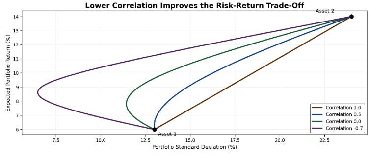
Figure 2 shows the same two assets combined under different assumed correlations. When correlation is +1.0, the risk-return relationship is a straight line because there is no diversification benefit. As correlation falls, the curve bends left, indicating lower risk for the same expected return. This is the visual foundation for why low or negative correlations are valuable in portfolio construction.

For an equally weighted portfolio in which all assets have the same variance and the same average correlation, the portfolio variance can be approximated as:

$$\sigma_P^2 = \frac{\sigma^2}{N} + \left( 1 – \frac{1}{N} \right) \bar{\rho} \sigma^2$$

Where:

• \(\sigma_P^2\) is the portfolio variance
• \(\sigma^2\) is the common asset variance
• \(N\) is the number of assets in the portfolio
• \(\bar{\rho}\) is the average correlation among the assets

As \(N\) becomes large, the first term becomes small and the covariance component dominates:

$$\sigma_P^2 \approx \bar{\rho} \sigma^2$$

Where:

• \(\sigma_P^2\) is the approximate variance of a large diversified portfolio
• \(\bar{\rho}\) is the average correlation among assets
• \(\sigma^2\) is the common asset variance

This result is important. Adding more assets reduces asset-specific risk, but it does not eliminate risk that comes from average co-movement. The portfolio can diversify away much unsystematic risk, but systematic risk remains.

Figure 3: Diversification Reduces Asset-Specific Risk, but Correlation Sets the Floor

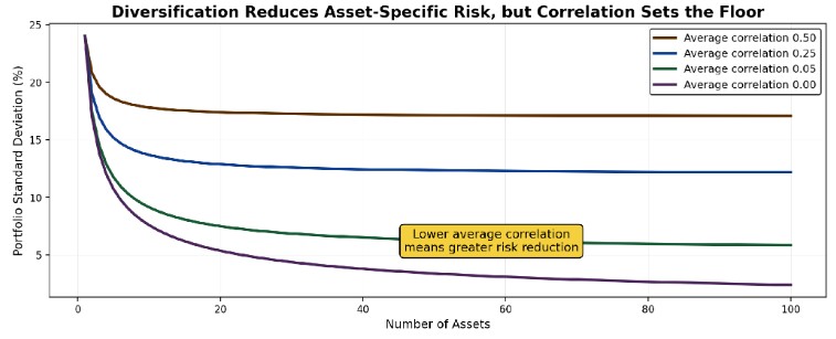
Figure 3 shows that adding assets initially reduces portfolio standard deviation quickly. After a point, however, the marginal benefit becomes smaller. The long-run level of risk depends heavily on average correlation. A portfolio of many highly correlated assets may still be risky, while a portfolio of lower-correlation assets can achieve a meaningfully lower risk level.

Example 7: Approximating the Risk of a Large Equal-Weighted Portfolio

Assume an analyst is evaluating a broad portfolio of 80 stocks. The average individual stock variance is estimated at 0.0625, and the average pairwise correlation is 0.18. Approximate the portfolio standard deviation.

Solution

Start by quoting the equal-variance approximation:

$$\sigma_P^2 = \frac{\sigma^2}{N} + \left( 1 – \frac{1}{N} \right) \bar{\rho} \sigma^2$$

Where:

• \(\sigma_P^2\) is the portfolio variance
• \(\sigma^2 = 0.0625\), the average individual asset variance
• \(N = 80\), the number of assets
• \(\bar{\rho} = 0.18\), the average pairwise correlation

Substitute the values:

$$\sigma_P^2 = \frac{0.0625}{80} + \left( 1 – \frac{1}{80} \right)(0.18)(0.0625)$$

$$\sigma_P^2 = 0.000781 + 0.011109 = 0.011891$$

Now calculate standard deviation:

$$\sigma_P = \sqrt{0.011891} = 10.90\%$$

For comparison, the large-portfolio approximation is:

$$ \begin{align*} \sigma_P^2 \approx \bar{\rho} \sigma^2 & = (0.18)(0.0625) = 0.01125 \\
\sigma_P \approx \sqrt{0.01125} & = 10.61\% \end{align*} $$

The approximation is close because the portfolio has many assets. Most of the portfolio risk is now driven by average covariance, not by the stand-alone variance of any single asset.

Evaluation Issues in Portfolio Statistics

Portfolio statistics should never be interpreted mechanically. A portfolio expected return may be historical or forward-looking. Historical estimates can be useful, but they may be biased if the past sample is short, stale, or unrepresentative. Forward-looking estimates can incorporate current valuations, economic conditions, and policy expectations, but they are still uncertain.

Covariances and correlations also change through time. In calm markets, certain assets may appear to diversify one another. During a crisis, correlations can rise as investors sell risky assets together. A risk model that assumes stable correlations may therefore understate risk precisely when diversification is most needed.

The analyst should also distinguish between portfolio risk and asset risk. Adding a volatile asset can reduce portfolio risk if it has sufficiently low correlation with the rest of the portfolio. Conversely, adding an apparently moderate-risk asset may increase total risk if it is highly correlated with existing exposures.

$$ \textbf{Table 3: Common Evaluation Traps in Portfolio Statistics} \\
\begin{array}{l|l|l}
\textbf{Trap} & \textbf{Why It Is Wrong} & \textbf{Better Interpretation} \\
\hline
\text{Treating expected return as a} & \text{Expected return is a forecast, not a} & \text{Evaluate the full distribution of} \\
\text{guaranteed outcome} & \text{certainty} & \text{possible outcomes} \\ \hline
\text{Averaging asset standard} & \text{Portfolio risk depends on} & \text{Use the portfolio variance formula} \\ \hline
\text{deviations to get portfolio risk} & \text{covariance and correlation} & \\
\text{Assuming correlation is stable} & \text{Correlations can change across} & \text{Stress test correlation assumptions} \\
& \text{regimes} & \\ \hline
\text{Believing diversification eliminates} & \text{Systematic risk cannot be} & \text{Diversification mainly reduces} \\
\text{all risk} & \text{diversified away} & \text{asset-specific risk} \\ \hline
\text{Ignoring portfolio drift} & \text{Weights change when assets} & \text{Monitor and rebalance when} \\
& \text{perform differently} & \text{needed} \\
\end{array} $$

Table 3 captures the judgment required by the word evaluate. The formulas are necessary, but the best investment analysts also ask whether the inputs are reliable and whether the result makes economic sense.

Interpretation and Evaluation

Several practical principles follow:

• Portfolio expected return is the weighted average of asset expected returns.
• Portfolio variance depends on asset weights, individual variances, and covariances.
• Portfolio standard deviation is the square root of portfolio variance.

• Covariance can be calculated from correlation and standard deviations.
• Correlation standardizes covariance and is easier to interpret.
• Lower correlation generally increases diversification benefits.
• Portfolio drift changes weights when assets earn different returns.
• Rebalancing helps control risk drift and style drift.
• In a large diversified portfolio, average covariance becomes more important than individual asset variance.
• Historical estimates should be used carefully when the future may differ from the past.

Question

A portfolio holds \(40\%\) in Asset A and \(60\%\) in Asset B. Asset A has an expected return of \(11\%\) and a standard deviation of \(22\%\). Asset B has an expected return of \(6\%\) and a standard deviation of \(10\%\). The correlation between the two asset returns is \(0.30\).

The portfolio’s expected return and standard deviation are closest to:

1. 8.00% and 12.05%
2. 8.00% and 14.80%
3. 9.00% and 12.05%

The correct answer is A.

Start by quoting the expected return formula:

$$E(r_P) = \sum_{i=1}^{N} w_i E(r_i)$$

Where:

• \(E(r_P)\) is the expected portfolio return
• \(w_A = 40\%\) and \(w_B = 60\%\), the portfolio weights
• \(E(r_A) = 11\%\) and \(E(r_B) = 6\%\), the expected returns
• \(N = 2\), the number of assets

The expected portfolio return is:

$$E(r_P) = (0.40)(11\%) + (0.60)(6\%) = 8.00\%$$

Now using the two-asset portfolio variance formula:

$$\sigma_P^2 = w_A^2 \sigma_A^2 + w_B^2 \sigma_B^2 + 2 w_A w_B \rho_{A,B} \sigma_A \sigma_B$$

Where:

• \(w_A = 40\%\) and \(w_B = 60\%\), the portfolio weights
• \(\sigma_A = 22\%\) and \(\sigma_B = 10\%\), the asset standard deviations
• \(\rho_{A,B} = 0.30\), the correlation between the two asset returns
• \(\sigma_P^2\) is the portfolio variance

Substitute the values:

$$\begin{align*}
\sigma_P^2 &= (0.40)^2(0.22)^2 + (0.60)^2(0.10)^2 + 2(0.40)(0.60)(0.30)(0.22)(0.10) \\
\sigma_P^2 &= 0.007744 + 0.003600 + 0.003168 = 0.014512
\end{align*}$$

The portfolio standard deviation is:

$$\sigma_P = \sqrt{0.014512} = 12.05\%$$

As such, the portfolio’s expected return is 8.00%, and the portfolio standard deviation is 12.05%.

B is incorrect because it overstates the standard deviation by adding a weighted average of asset standard deviations rather than applying the portfolio variance formula.

C is incorrect because it overstates the expected return by reversing the portfolio weights.