Explain Inflation, Hyperinflation, Dis ...
Inflation Inflation is the persistent increase in the general price level of goods... Read More
An optimal price can be defined as the price at which a seller can make the highest profit possible; that is, the seller’s price is maximized. The rule of marginal output postulates that profit is maximized by producing an output, whereby the marginal cost (MC) of the last unit produced is exactly equal to the marginal revenue (MR). Simply put, MC=MR.
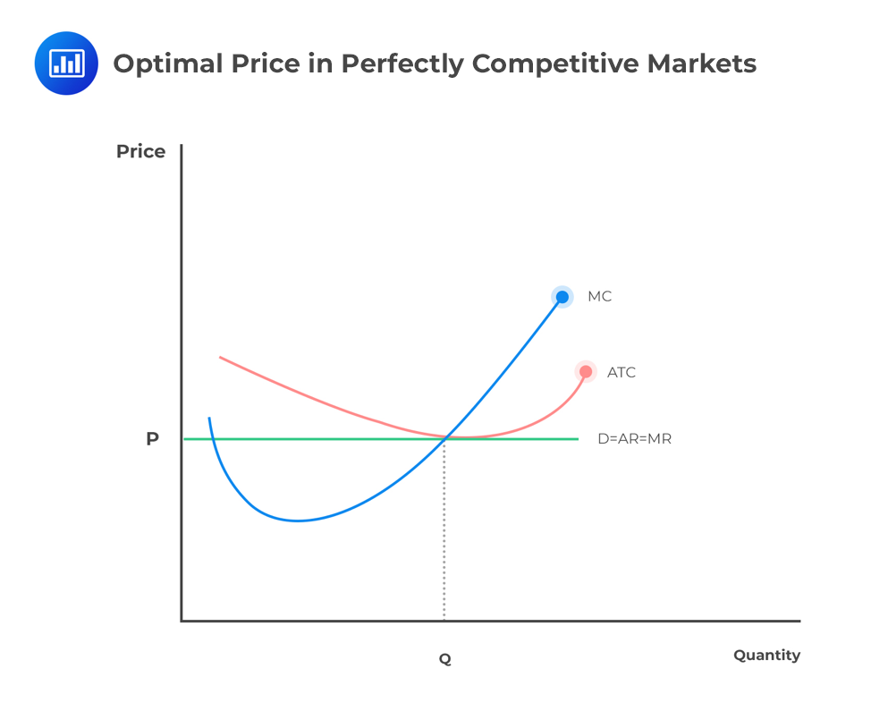
Under perfect competition, there are many firms in the market. If one firm decides to increase production, the market equilibrium price won’t be highly affected. Conversely, if a single firm changes the market price at equilibrium, then the market won’t be in perfect competition. Therefore, each firm faces a demand curve that is horizontal at equilibrium.
In perfect competition, any profit-maximizing producer has a market price equal to its marginal cost (P=MC).

If the price function P = 20 – Q, and MC = 5 + 2Q, calculate the profit-maximizing price and output.
The profit is maximized when:
\(P = MC \Rightarrow 20 – Q = 5 + 2Q\)
\(\therefore 3Q=15 \Rightarrow Q=5\)
Substituting Q into the price function:
\(P = 20 – 5 = 15\)
The profit-maximizing price and output are 15 and 5, respectively.
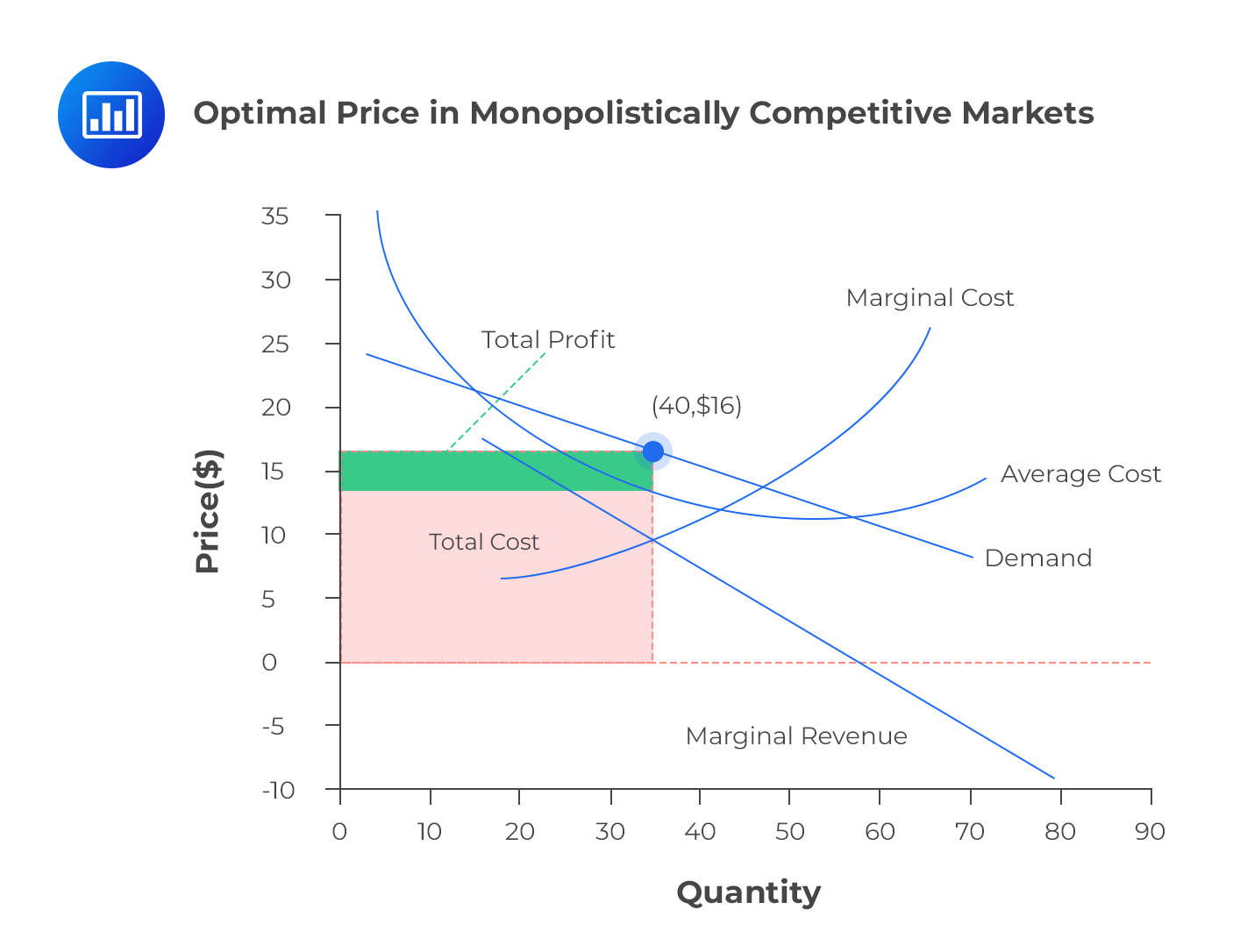
In this market structure, the short-run profit-maximizing choice occurs at the point where marginal revenue is equal to marginal cost (MR=MC). Total revenue (TR) is a product of price and quantity:
$$TR = P\times Q$$
The average cost incurred in producing Q units of a product is taken as C. Therefore, the total cost (TC) is calculated as the product of average cost and total quantity. That is,
$$TC = C\times Q$$
The economic profit is the difference between TR and TC. We denote the economic profit by π. Then,
$$\pi= TR-TC$$

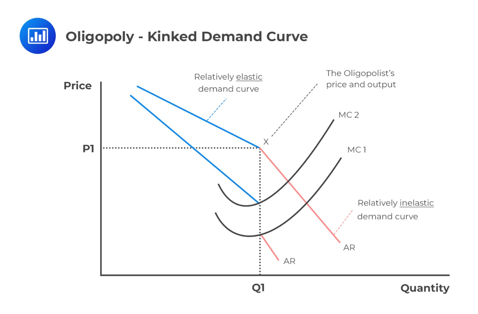
There is no well-defined optimal price and optimal output in this market structure. In fact, this has already been discussed in the previous learning objective about the supply function of an oligopolistic market. There exist many firms that form an oligopoly. These firms all have their own pricing models. When there exists a kinked curve, the optimal price is taken at the point of the kink. However, the kinked demand curve can’t explain the cause of that kink.

In the case of a dominant firm, the output level is vital in determining the optimal price. This occurs at the point where MR = MC. The profit-maximizing price is thus calculated by that segment of the demand function that the dominant firm faces.
Moreover, when we have a Cournot model (in which companies compete on the amount of output they will produce), every firm assumes that the other firms cannot alter their price levels of output with respect to the dominant firm. Their optimum price is still at MR = MC.
In a Nash equilibrium (no participant can gain by a unilateral change of strategy), firms react to their own circumstances and maximize their own profits. This continues until each firm is independently stable.
The combination of output and price that maximizes profit occurs at the elastic portion of the demand curve. This is because MR and MC will always intersect at the point where MR is positive. In this case, demand is elastic when MC = MR. The relationship between MR and price elasticity,\(E_p\), is
$$MR=P[1-\frac{1}{E_p}]$$
In a monopoly, MR = MC thus:
$$MR=P[1-\frac{1}{E_p}]=MC$$
A firm informed of its cost structure and its price elasticity(\(E_p\)) can use this relationship to work out its profit-maximizing price.
The marginal cost(MC) of a production company is $100. From the past market analysis, the price elasticity was approximated to be 1.5. Calculate the optimal price.
Using the equation,
\(P[1-\frac{1}{E_p}]=MC\)
\(\Rightarrow P[1-\frac{1}{1.5}]=100 \therefore P=300\)
Question
A firm that is operating in a monopolistically competitive market environment maximizes its profits when:
- the average cost is minimized.
- marginal revenue equals average cost.
- marginal revenue equals marginal cost.
Solution
The correct answer is C.
The firm will maximize its profit when the level of output is such that, the marginal revenue equals marginal cost. In other words, it will produce the quantity such that MR=MC.
A and B are incorrect. From the graph given below, we can clearly see that it’s neither the point where average cost is minimized nor the point where marginal revenue equals average cost.
Get Ahead on Your Study Prep This Cyber Monday! Save 35% on all CFA® and FRM® Unlimited Packages. Use code CYBERMONDAY at checkout. Offer ends Dec 1st.