Sharpe Ratio, Treynor Ratio and Jensen’s Alpha (Calculations for CFA® and FRM® Exams)

Portfolio Performance Measures

Portfolio management involves a trade-off between risk and return. Most amateur investors mistakenly focus only on the return aspect and lose sight of the risk taken to achieve the return. The portfolio performance measures are intended as metrics to compare different portfolios quickly. Like any financial ratio, these are not intended to be a one-stop answer to decide on a portfolio and should instead be used in conjunction with other data points.

The measure themselves are quite different from one another in the way that they measure the trade-off and how they define risk.

Sharpe Ratio

The Sharpe Ratio is defined as the portfolio risk premium divided by the portfolio risk:

$$ \text{Sharpe ratio} = \frac{\text{Return on the portfolio} – \text{Return on the risk-free rate}}{\text{Standard deviation of the portfolio}} = \frac{R_p – R_f}{σ_p} $$

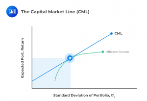
The Sharpe ratio, or reward-to-variability ratio, is the slope of the capital allocation line (CAL). The greater the slope (higher number) the better the asset.

Note that the risk being used is the total risk of the portfolio, not its systematic risk, which is a limitation of the measure. The portfolio with the highest Sharpe ratio has the best performance, but the Sharpe ratio by itself is not informative. In order to rank portfolios, the Sharpe ratio for each portfolio must be computed.

A further limitation occurs when the numerators are negative. In this instance, the Sharpe ratio will be less negative for a riskier portfolio resulting in incorrect rankings.

Example: Calculating the Sharpe Ratio     

A client has three portfolio choices, each with the following characteristics:

The efficient market portfolio has an expected return of 20% and a standard deviation of 12%, and the risk-free rate of interest is 5%.

Based on the Sharpe ratio for each portfolio, the client should choose:

A. Portfolio A

B. Portfolio B

C. Portfolio C

Solution

The correct answer is B.

\( \text{Sharpe ratio} = \frac{\text{Return on the portfolio} – \text{Return on the risk-free rate}}{\text{Standard deviation of the portfolio}} = \frac{R_p – R_f}{σ_p} \)

\(\text{Portfolio A’s Sharpe Ratio} = \frac{15\%−5\%}{12\%} = 0.83\)

\(\text{Portfolio B’s Sharpe Ratio} = \frac{18\%−5\%}{14\%} = 0.93\)

\(\text{Portfolio C Sharpe Ratio} = \frac{12\%−5\%}{9\%} = 0.77\)

The client should choose portfolio B as it gives the highest Sharpe ratio.

Type of Risks

The Sharpe Ratio defines the risk in terms of standard deviation, which is a measure of total risk. Hence, it includes both systematic as well as unsystematic risk. The next measures that we look at – Treynor Ratio and Jensen’s Alpha – define the risk in a narrower way. In order to understand the applicability of the measure, we first need to understand the different types of risks.

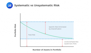
CAPM suggests that investors should hold the market portfolio and a risk-free asset. The true market portfolio consists of a large number of securities, and it may not be practical for an investor to own them all. Much of the non-systematic risk can be diversified away by holding 30 or more individual securities. However, these securities should be randomly selected from multiple asset classes. An index may serve as the best method of creating diversification.

It is important to note that only non-systematic risk can be eliminated through the addition of different securities into the portfolio. Systematic risk – the risk inherent to the entire market – cannot be diversified away.

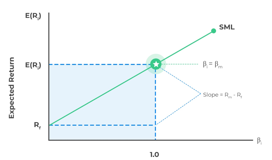
The systematic risk of a portfolio is denoted by Beta:

$$ β_i = \frac{\text{Covariance  between the security and the market}}{\text{Variance of the Market}} = \frac{Cov(R_i, R_m)}{σ_m^2} $$

Example: Calculating the Expected Return of a Security

Assume the risk-free rate is 2%, security has a correlation of 0.8 with the market index and a standard deviation of 16% while the standard deviation of the market is 12%. If the market expected return is 8%, what is the expected return of the security?

A. 10.56%

B. 5.60%

C. 8.42%

Solution

The correct answer is C.

$$ E(R_i)=R_f+β_i[E(R_m)–R_f] $$

Where

\(E(R_i)\) = the expected return of asset i over the holding period.

\(R_f\)  = rate of return on the risk-free asset.

\(R_m\) = Expected market return over the holding period.

\(ꞵ_i\) = the Beta factor of the asset i.

Note that \((R_m-R_f)\) is the expected return per unit risk (beta) and \(ꞵ_i(R_m-R_f)\) is the expected return above the risk-free rate of return.

Step 1: Find the Beta

\(ꞵ_i= \frac{0.8 × 0.16\times 0.12}{0.12^2}  = 1.07\)

Step 2: Find the expected return

\(E(R_i) = 2\% + 1.07 × (8\% – 2\%) = 8.42\%\)

FRM Part I & Part II Complete Course

Treynor Ratio

The Treynor ratio is an extension of the Sharpe ratio that, instead of using total risk, uses beta or systematic risk in the denominator. As such, this is better suited to investors who hold diversified portfolios.

$$ \text{Treynor ratio} = \frac{\text{Return on the portfolio} – \text{Risk-free rate}}{\text{Beta of the portfolio}} = \frac{R_p – R_f}{B_p} $$

As with the Sharpe ratio, the Treynor ratio requires positive numerators to give meaningful comparative results and, the Treynor ratio does not work for negative beta assets. Also, while both the Sharpe and Treynor ratios can rank portfolios, they do not provide information on whether the portfolios are better than the market portfolio or information about the degree of superiority of a higher ratio portfolio over a lower ratio portfolio.

Example: Calculating Treynor’s Ratio

A portfolio manager earned an average annual return of 12%. The beta of the portfolio is 0.9, and the volatility of returns is 25%. The average annual return for the market index was 14%, and the standard deviation of the market returns is 30%. The risk-free rate is 5%. Calculate the Treynor measure for the portfolio.

A. 10.0%

B. 5.6%

C. 7.8%

Solution

The correct answer is C:

Formula:$$\frac{R_p – R_f}{B_p}$$

$$=\frac{12\%−5\%}{9\%} = 7.8%\)$$

Jensen’s Alpha

Jensen’s Alpha is based on systematic risk. The daily returns of the portfolio are regressed against the daily returns of the market in order to compute a measure of this systematic risk in the same manner as the CAPM. The difference between the actual return of the portfolio and the calculated or modeled risk-adjusted return is a measure of performance relative to the market.

$$ { \alpha }_{ \text{P} }={ \bar { \text{R} } }_{ \text{p} }-\left( { \bar { \text{R} } }_{ \text{f} } +{ \beta }_{ \text{p} }\left( { \bar { \text{R} } }_{ \text{m} }-{ \bar { \text{R} } }_{ \text{f} } \right)\right) $$

If \(α_p\) is positive, the portfolio has outperformed the market, whereas a negative value indicates underperformance. The values of Alpha can also be used to rank portfolios or the managers of those portfolios, with the Alpha being a representation of the maximum an investor should pay for the active management of that portfolio.

Example: Calculating Jensen’s Alpha

Two portfolios have the following characteristics:

Given a market return of 10% and a risk-free rate of 4%, calculate Jensen’s Alpha for both portfolios and comment which portfolio has performed better.

A. -0.2%  and -3.6% respectively; Portfolio A has performed better than Portfolio B.

B. -0.2% and -3.6% respectively; Portfolio B has performed better than Portfolio A.

C. 0.2% and 3.6% respectively; Portfolio B has performed better than Portfolio A.

Solution

The correct answer is A.

$$ \text{Jensen’s alpha } ({ \alpha }_{ \text{P} })={ \bar { \text{R} } }_{ \text{p} }-\left( { \bar { \text{R} } }_{ \text{f} } +{ \beta }_{ \text{p} }\left( { \bar { \text{R} } }_{ \text{m} }-{ \bar { \text{R} } }_{ \text{f} } \right)\right) $$

\(\text{Jensen’s Alpha for Portfolio A} = 0.08 – [0.04 + 0.7(0.1 – 0.04)] = -0.002\)

\(\text{Jensen’s Alpha for Portfolio B} = 0.07  – [0.04 + 1.1(0.1 – 0.04)] = -0.036\)

Jensen’s Alpha is -0.2% and -3.6% for portfolios A  and B, respectively. A higher Jensen’s Alpha (-0.2% in this case) indicates that a portfolio has performed better. Also note that both portfolio managers have been unable to create Alpha, but the manager of portfolio A has been not as bad as portfolio B’s manager.