The covariance is a measure of the degree of co-movement between two random variables. For instance, we could be interested in the degree of co-movement between the variables X and Y, where we can let:

• X = interest rate
• Y = inflation

The general formula used to calculate the covariance between two random variables, X and Y, is:

$$COV\ [X,\ Y] =E[(X-E[X]) (Y-E[Y])]$$

Where:

\(X\) = a random variable such as lending interest rates.

\(Y\) = another random variable, such as inflation rates.

\(E[X]\) = The expected value (mean) of X.

\(E[Y]\) = The expected value (mean) of Y.

The covariance between two random variables can be positive, negative, or zero.

• A positive number indicates co-movement (i.e., the variables tend to move in the same direction);
• A value of zero indicates no relationship; and
• A negative value shows that the variables move in opposite directions.

Moreover, if variables are independent, their covariance is zero, i.e.,

$$COV\left(X,Y\right)=E\left(XY\right)-E\left(X\right)E\left(Y\right)=0$$

Covariances can be represented in a tabular format in a covariance matrix as follows:

$$ \begin{array}{c|ccc} \text{Asset} & A & B & C \\ \hline A & \text{Cov}(A, A) & \text{Cov}(A, B) & \text{Cov}(A, C) \\ B & \text{Cov}(B, A) & \text{Cov}(B, B) & \text{Cov}(B, C) \\ C & \text{Cov}(C, A) & \text{Cov}(C, B) & \text{Cov}(C, C) \\ \end{array} $$

• The off-diagonal terms represent variances since, for example, \(\text{Cov(C, C) = Var(C)}\)
• A two-asset portfolio would have a similar 2 × 2 matrix.
• A correlation matrix can also be created to represent the correlations between various assets in a large portfolio.

Example 1: Calculating the Covariance of a Portfolio of Two Assets

A portfolio comprises two stocks – 1 and 2. The returns for the last 5 years are as follow:

Stock 1: 5%; 4.5%; 4.8%; 5.5%; 6%.

Stock 2: 6%; 6.2%; 5.7%; 6.1%; 6.5%.

Compute the covariance.

Solution

Step 1: We calculate the weighted sum of each stock to get the expected return on Stock 1 and Stock 2

$$\begin{align} E(R_1)& = \frac{5\%+4.5\%+4.8\%+5.5\%+ 6\%}{5} = 5.2\% \\ E(R_2) &= \frac{6\%+ 6.2\%+ 5.7\%+ 6.1\%+ 6.5\%}{5} = 6.1\% \end{align}$$

Step 2: We subtract each year’s return from the expected return to obtain [R1-E(R1)] and [R2-E(R2)] as follows:

$$ \begin{array}{c|c|c|c|c} \textbf{Year} & R_1 & R_2 & R_1 – \mathbb{E}(R_1) & R_2 – \mathbb{E}(R_2) \\ \hline 1 & 5\% & 6\% & -0.2\% & -0.1\% \\ 2 & 4.5\% & 6.2\% & -0.7\% & 0.1\% \\ 3 & 4.8\% & 5.7\% & -0.4\% & -0.4\% \\ 4 & 5.5\% & 6.1\% & 0.3\% & 0\% \\ 5 & 6\% & 6.5\% & 0.8\% & 0.4\% \\ \end{array} $$

Step 3: We multiply the values obtained in Step 2 and we divide by the number of observations to get a mean observation.

$$\begin{align}
\text{Cov}(R_1, R_2) &= \mathbb{E}[(R_1 – \mathbb{E}[R_1])(R_2 – \mathbb{E}[R_2])] \\
&= \frac{
\begin{array}{l}
(-0.002 \times -0.001) + (-0.007 \times 0.001) + \\
(-0.004 \times -0.004) + (0.003 \times 0) + (0.008 \times 0.004)
\end{array}
}{5} \\
&= \frac{0.000002 + (-0.000007) + 0.000016 + 0 + 0.000032}{5} \\
&= \frac{0.000043}{5} = 0.0000086
\end{align}$$

Example 2: Covariance

Consider a set of a well-diversified portfolios X and Y. Suppose that the mean returns for X and Y are 6.12 and 7.04, respectively, what is the covariance between these portfolios?

Solution

Recall,

$$COV\left(X,Y\right)=E\left(XY\right)-E\left(X\right)E\left(Y\right)\)$$

For independent variables,

$$E\left(XY\right)=E\left(X\right)E\left(Y\right)=6.12\times7.04=43.0848$$

Which implies that,

$$COV\left(X,Y\right)=E\left(XY\right)-E\left(X\right)E\left(Y\right)=43.0848-6.12\left(7.04\right)=0$$

Correlation

Correlation is the ratio of the covariance between two random variables and the product of their two standard deviations i.e.

$$\text{Correlation}\ (X_1,X_2\ )=\frac{Cov(X_1,X_2\ )}{\text{Standard deviation}\ (X_1\ )\times \text{Standard deviation}\ (X_2\ )}$$

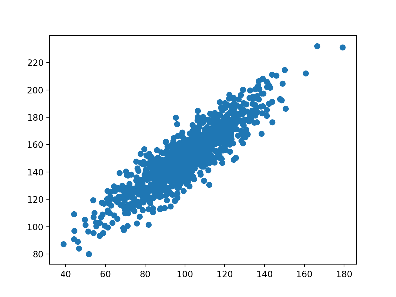
Correlation measures the strength of the linear relationship between two variables. While the covariance can take on any value between negative infinity and positive infinity, the correlation is always a value between -1 and +1.

A correlation of -1 indicates a perfect inverse relationship (i.e. a unit change in one means that the other will have a unit change in the opposite direction). Secondly, a correlation of +1 indicates a perfect linear relationship (i.e. the two variables move in the same direction with the unit changes being equal). Finally, a correlation of zero implies that there is no linear relationship between the variables.

Example: Calculating the Covariance

We anticipate that there is a 15% chance that next year’s stock returns for ABC Corp will be 6%, a 60% probability that they will be 8% and a 25% probability that they will be 10%. We already know the expected value of returns is 8.2% and the standard deviation is 1.249%.

We also anticipate that the same probabilities and states are associated with a 4% return for XYZ Corp, a 5% return, and a 5.5% return. The expected value of returns is then 4.975 and the standard deviation is 0.46%.

$$ \begin{align}
\text{cov}(\text{R}_{ \text{ABC}},\text{R}_{ \text{XYZ}}) & = 0.15(0.06 – 0.082)(0.04 – 0.04975) \\
& + 0.6(0.08 – 0.082)(0.05 – 0.04975) \\
& + 0.25(0.10 – 0.082)(0.055 – 0.04975) \\
& = 0.0000561 \\
\end{align} $$

Recall that,

$$\text{Corr}(\text{R}_{ \text{ABC}},\text{R}_{ \text{XYZ}})=\frac{\text{Cov}(\text{R}_{ \text{ABC}},\text{R}_{ \text{XYZ}}\ )}{(\text{Standard deviation}\ (\text{R}_{ \text{ABC}}\ )\times \text{Standard deviation} (\text{R}_{ \text{XYZ}}\ ))}$$

Thus,

$$\text{Correlation}=0.0000561\left(0.01249\times0.0046\right)=0.976$$

Interpretation: The correlation between the returns of the two companies is very strong (almost +1) and the returns move linearly in the same direction.

All 3 Levels of the CFA Exam – Complete Course offered by AnalystPrep

How does Correlation Impact Portfolio Risk?

As mentioned earlier, correlation ranges from -1 to +1

• +1 = returns are perfectly positively correlated.
• 0 = returns of two assets are not correlated.
• -1 = returns are perfectly negatively correlated.
• What happens to portfolio risk (in a portfolio of two risky assets) when the two assets are perfectly correlated?
• Risk is unaffected; no benefit of diversification

In conclusion, using negatively correlated investments to form a portfolio helps to reduce the overall volatility of the portfolio.

Ready to Apply These Formulas?

Understanding the formulas is one thing—mastering them under exam pressure is another. Put your knowledge to the test with AnalystPrep’s CFA Level 1 practice questions. You’ll get access to hundreds of quant-focused problems, detailed solutions, and performance tracking tools to help you study smarter.

CFA Level I Practice Questions

FAQs on Covariance and Correlation

1. What is the covariance formula for CFA Level 1?

The formula for covariance between two random variables \( X \) and \( Y \) is:

\[ \text{Cov}(X, Y) = \mathbb{E}\left[(X – \mathbb{E}[X])(Y – \mathbb{E}[Y])\right] \]

Alternatively:

\[ \text{Cov}(X, Y) = \mathbb{E}[XY] – \mathbb{E}[X]\mathbb{E}[Y] \]

Where:

• \( X, Y \) = Random variables (e.g., returns, interest rates)
• \( \mathbb{E}[X], \mathbb{E}[Y] \) = Expected values (means) of \( X \) and \( Y \)
• \( \mathbb{E}[XY] \) = Expected value of the product \( XY \)

2. What’s the difference between covariance and correlation?

Covariance indicates the direction of co-movement between two variables but is affected by the units of measurement. Correlation standardizes this to a scale from -1 to +1.

\[ \rho(X, Y) = \frac{\text{Cov}(X, Y)}{\sigma_X \cdot \sigma_Y} \]

Where:

• \( \rho(X, Y) \): Correlation between \( X \) and \( Y \)
• \( \text{Cov}(X, Y) \): Covariance between \( X \) and \( Y \)
• \( \sigma_X, \sigma_Y \): Standard deviations of \( X \) and \( Y \), respectively

3. How do I convert covariance to correlation?

Use the correlation formula to convert covariance to a dimensionless metric:

\[ \text{Correlation} = \frac{\text{Cov}(X, Y)}{\sigma_X \cdot \sigma_Y} \]

Where:

• \( \text{Cov}(X, Y) \): Covariance between the two variables
• \( \sigma_X \): Standard deviation of variable \( X \)
• \( \sigma_Y \): Standard deviation of variable \( Y \)

4. Why is a correlation of zero not the same as independence?

A correlation of zero means there’s no linear relationship between variables, but they may still be dependent in other ways. Independence is a much stronger condition.

$$\begin{align}\rho(X, Y) = 0 &\Rightarrow \text{No linear relationship} \\ \text{Cov}(X, Y) = 0 & \Rightarrow \text{Independence} \end{align}$$

However, the converse is not always true: zero covariance does not imply independence unless the variables are jointly normally distributed.

5. How does correlation affect portfolio risk?

The correlation between assets determines the potential for diversification in a portfolio. The lower the correlation, the greater the risk-reduction benefit.

• \( \rho = +1 \): Perfect positive correlation – no diversification benefit
• \( \rho = 0 \): No linear relationship – some diversification benefit
• \( \rho = -1 \): Perfect negative correlation – maximum diversification benefit

In general, combining negatively or weakly correlated assets helps reduce portfolio volatility.