Corporate Finance – Level I CFA® Program Essential Review Summary offered by AnaystPrep

Reading 31 – Introduction to Corporate Governance and ESG Considerations

Corporate Governance is the managerial system by which a company is controlled. There are two primary theories that drive corporate governance structures, though they have been converging more closely together in their influence more recently. The Shareholder Theory operates under the assumption that the most important responsibility of company management is to maximize returns to shareholders. The Stakeholder Theory emphasizes the needs of all relevant stakeholders in making decisions about the company’s operations. These additional stakeholders include customers, employees, and even suppliers and creditors.

There are a variety of stakeholder groups connected to a company that will have different interests in the company’s results. Creditors provide debt financing and are primarily concerned with the company being able to keep up with interest and principal payments. They are less concerned about the growth upsides because they do not benefit beyond debt repayments. Equity Shareholders are the owners of the company and stand to benefit from all future growth the company experiences. Shareholders typically have voting rights regarding major company decisions, including membership in the Board of Directors. Managers and Employees are impacted by both the upside and downside risks of a company. Customers are less concerned with the operations of the company itself and more about the value they receive when they purchase goods and services.

Companies must work to manage their relationships with stakeholders. Annual meetings with shareholders are typically held shortly after financial statements are published so that results and concerns can be addressed by company management. Extraordinary shareholder meetings can also be held when there are major resolutions that require a certain threshold of shareholder approval. The shareholders’ interests are represented by the Board of Directors, who oversee the company management and are elected by the shareholders. Companies are also subject to audit controls, both by independent internal audit groups and external auditors.

Factors that can affect stakeholder relationships fall into two categories: Market and Non-Market factors. Market factors relate to capital markets and include shareholder engagement through annual meetings, shareholder activism in which large holders try to force changes in the company’s strategy to increase shareholder value, and takeovers in which shareholders try to change the company’s structure to take advantage of opportunities with other companies. Non-market forces that can have a major impact include the legal environment in which the company does business, media and the quick spread of news and opinions (especially social media), and the growth of the corporate governance industry itself.

Poor corporate governance can pose significant risks to a company’s success. Managers with too little oversight can make short-sighted decisions that benefit themselves at the expense of shareholders. One stakeholder group could benefit unfairly at the expense of another due to a lack of proper controls. The company could be exposed to legal, regulatory, or reputational risks that could include financial penalties and loss of business.

Several factors that have been gaining in importance for companies throughout the world are what is known as ESG, which stands for Environmental, Social, and Governance. ESG analysis includes looking at factors that may not have historically been included in research done about companies, but represent items that are important to a broader set of stakeholders of all companies. This analysis is often done by using screeners on these criteria to exclude companies with weak policies or histories on these factors from potential investment decisions.

Reading 32 – Capital Budgeting

Capital budgeting is the process by which companies make decisions on projects with a lifespan of one year or more. It involves comparing the costs and benefits of one or multiple long-term projects in order to best allocate the resources of the company. There are four primary steps in the capital budgeting process:

1. Generate ideas for potential projects
2. Analyze individual project proposals based on forecasted cash flow and profitability
3. Plan the capital budget
4. Monitor and post-audit during and after the project

There are several categories of capital budgeting project. Replacement Projects involve replacing worn down equipment or switching to newer, more efficient machinery and processes. Expansion Projects increase the size of a company’s business activities. New Products expand a company’s product or service offerings. Regulatory, Safety, and Environmental Projects are usually undertaken due to external requirements by regulators or government agencies.

Capital budgeting decisions are based on cash flows rather than accounting earnings. The timing of these cash flows is critical and are always analyzed on an after-tax basis. The opportunity costs of these cash flows is a major component of the analysis and decision-making process. Financing costs are ignored because they are reflected in the required rate of return.

An important concept in capital budgeting is that of Sunk Costs. These are costs that have already been incurred and should not have significant impacts on future spending decisions. Opportunity Costs represent the value of the next best use of a resource. Externalities are effects of an investment outside of the investment itself. An example of this would be the cannibalization of business from one unit to another due to an expansion project.

Capital budgeting decisions are impacted by the nature of the projects under analysis. Often, projects may be Mutually Exclusive and you will need to choose only one from a set of choices due to limitations on resources. Project Sequencing is another important concept, in that some projects may create opportunities for other projects in future that might not otherwise be available. Capital Rationing occurs when there are fixed or limited resources available for investment in potential projects. Many exam questions in this area will ask you to choose the best investment opportunity, given a limited capital budget.

The quantitative methods of capital budgeting are related to material covered in the Quantitative Methods section. The two most common measurements are Net Present Value (NPV) and Internal Rate of Return (IRR).

$$ NPV=\sum _{ }^{ }{ \frac { { CF }_{ t } }{ { \left( 1+r \right) }^{ t } } }
$$
$$ { CF }_{ t }=cash\quad flow\quad at\quad time\quad t $$
$$ r=required\quad rate\quad of\quad return $$
Depending on when there are cash outflows or inflows, the total cash flows in each period can be positive or negative. If the NPV is positive, then the project will increase company profitability. When comparing multiple projects by NPV, the larger NPV is the better option.

The IRR is the rate of return at which NPV is equal to 0. It is a way of calculating the rate of profitability of a capital project. A higher IRR is preferable. When the IRR and NPV metrics give conflicting information about which project should be chosen, use the one with the highest NPV.

Small projects can have high IRRs but not provide as much value to the company, so the NPV is a better comparison of the overall scale of the return.

Another metric used for capital budgeting projects is the Payback Period. This is simply the number of years it takes for a project to pay back its initial investment. A more advanced version of this is the Discounted Payback Period. This is the same formula, but it discounts the future cash flows back to a present value in order to determine how long it will take to pay back its investment.

The final measurement for comparing capital projects is the Profitability Index. This is the ratio of a project’s discounted cash flows to its initial investment. A profitability index greater than 1 is an indication that it’s a good investment.

$$ PI=\frac { PV\quad of\quad future\quad cash\quad flows }{ Initial\quad investment } =1+\frac { NPV }{ Initial\quad investment } $$

Reading 33 – Cost of Capital

The cost of capital is the price to a company for investment resources. For a company to remain in business and grow over time, it must be able to earn more from its projects and operations than it spends to get that capital. The cost of capital to the firm is not observable, but must be estimated using assumptions about the marginal cost of additional funding. Since a company can have many sources of capital funding, the common metric used is the Weighted Average Cost of Capital, which incorporates all possible sources of new marginal capital.

$$ WACC={ w }_{ d }{ r }_{ d }\left( 1-t \right) +{ w }_{ p }{ r }_{ p }+{ w }_{ e }{ r }_{ e } $$

The three components of WACC are Debt, Preferred stock, and Equity. The formula combines the proportion and rate of each component to create a summary figure that applies to the firm as a whole. The rate applied to debt is multiplied by 1-the marginal tax rate because interest payments on debt are tax-deductible. The proportions of each component are the market value of that component divided by the sum of the market value of all three capital components (done correctly, they should always sum to 100%).

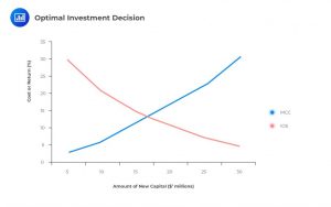
There is a relationship that exists in determining the optimal amount of capital a company should take on to pursue new investment opportunities. As a company accumulates more capital, it will face increasing costs on each additional capital amount while it will also face decreasing returns on new projects. This relationship is highlighted in the graph below:

Companies can also adjust their cost of capital assumptions to account for higher or lower levels of risk in potential projects.

When trying to calculate the cost of debt financing, there are two primary approaches. The Yield-to-Maturity Approach is the yield that equates the present value of the bond’s future payments to its market price.

$$ { P }_{ 0 }=\left( \sum _{ }^{ }{ \frac { { PMT }_{ t } }{ { \left( 1+\frac { { r }_{ d } }{ 2 } \right) }^{ t } } } \right) +\frac { FV }{ { \left( 1+\frac { { r }_{ d } }{ 2 } \right) }^{ n } } $$
$$ { P }_{ 0 }=current\quad market\quad price\quad of\quad bond $$
$$ { PMT }_{ t }=interest\quad payment\quad in\quad period\quad t $$
$$ { r }_{ d }=the\quad yield\quad to\quad maturity $$
$$ n=number\quad of\quad periods\quad remaining\quad to\quad maturity $$
$$ FV=the\quad maturity\quad value\quad of\quad the\quad bond $$

The Debt-Rating Approach uses the yield on similar debt securities when accurate market price data for a company’s debt is not available. The applicable yield is equal to the stated yield of the debt instrument multiplied by 1 minus the marginal tax rate. It’s important to remember that the rate on debt capital is always net of tax.

Preferred Stock is the second component that a company could use to raise capital. These shares represent different claims of ownership on the company than common equity. They typically offer higher (and often fixed) dividend rates and usually have no voting rights. The cost of these to the company is simply the dividend yield on the shares:

$$ { r }_{ p }=\frac { { D }_{ p } }{ { P }_{ p } } $$
$$ { r }_{ p }=rate\quad of\quad preferred\quad stock $$
$$ { D }_{ p }=preferred\quad stock\quad dividends\quad per\quad share $$
$$ { P }_{ p }=preferred\quad stock\quad price\quad per\quad share $$

Common Equity is the third component of a company’s capital base. A company can increase its common equity by reinvesting earnings or issuing new stock. The cost of equity capital is the required rate of return to the shareholders. There are three methods of calculating the cost of equity. The first is the Capital Asset Pricing Model:

$$ E\left( { R }_{ i } \right) ={ R }_{ f }+\beta \left[ E\left( { R }_{ m } \right) -{ R }_{ f } \right] $$
$$ E\left( { R }_{ i } \right) =cost\quad of\quad equity $$
$$ { R }_{ f }=risk\quad free\quad interest\quad rate $$
$$ { \beta }_{ i }=equity\quad beta $$
$$ E\left( { R }_{ m } \right) =expected\quad market\quad return $$

The second is the Dividend Discount Model, which is based on the assumption that a stock’s intrinsic value is the present value of its expected future dividends:

$$ { r }_{ e }=\frac { { D }_{ 1 } }{ { P }_{ 0 } } +g $$
$$ { P }_{ 0 }=current\quad share\quad price $$
$$ { D }_{ 1 }=dividend\quad due\quad next\quad period $$
$$ { r }_{ e }=cost\quad of\quad equity $$
$$ g=dividend\quad growth\quad rate $$

The third method is the Bond Yield plus Risk Premium Approach. This involves adding an equity risk premium to the company’s bond yield to estimate the cost of equity.

In some instances, it may be necessary to add an additional risk premium. One such example is for companies operating in developing or otherwise risky countries where the equity premium does not fully capture the extra risk required by equity investors. A country-specific risk premium can be calculated as follows:
$$ \begin{matrix} Country\quad risk \\ premium \end{matrix}=\begin{matrix} Sovereign\quad yield \\ spread \end{matrix}\times \frac { \begin{matrix} Annualized\quad standard\quad deviation\quad of\quad \\ equity\quad index \end{matrix} }{ \begin{matrix} Annualized\quad standard\quad deviation\quad of\quad sovereign\quad \quad \\ bond\quad market\quad in\quad terms\quad of\quad the\quad developed \\ market\quad currency \end{matrix} } $$

Reading 34 – Measures of Leverage

Companies face uncertainty around the operational results and the investments that are made in the hopes of leading to growth in the future. Leverage is the use of increased fixed costs that are intended to help increase company growth. Companies with high amounts of leverage will experience greater variation in net income and have more volatile earnings and cash flows. There are several types of risk associated with leverage. Financial Risk is associated with how the company acquires capital (i.e., debt vs equity) to fund its operations. Business Risk is the risk inherent in a company’s core operations. Sales Risk is the uncertainty associated with the price and quantity of goods and services a company offers for sale. Operating Risk is attributed to the part of a company’s operating structure related to its use of fixed costs.

There are three important ratios to help quantify types of risk associated with leverage. The Degree of Operating Leverage (DOL) measures how sensitive a company’s operating income is to changes in sales. The formula highlights the amounts related specifically to fixed costs:

$$ DOL=\frac { Q\left( P-V \right) }{ Q\left( P-V \right) -F } $$
$$ Q=units\quad sold $$
$$ P=unit\quad price $$
$$ V=variable\quad cost\quad per\quad unit $$
$$ F=fixed\quad cost\quad per\quad unit $$

The Degree of Financial Leverage (DFL) refers to the sensitivity of the operating income of a company to changes in earnings.

$$ DFL=\frac { Q\left( P-V \right) -F }{ Q\left( P-V \right) -F-C } $$

The Degree of Total Leverage (DTL) combines both previous formulas to provide the sensitivity of net income to changes in units sold.

$$ DTL=\frac { Q\left( P-V \right) }{ Q\left( P-V \right) -F-C } $$

Higher degrees of financial leverage can cause a drag on earnings due to higher amounts of financial interest payments. When used properly, the leverage leads to increases in earnings and cash flows when the company is doing well. A company with more leverage is, however, always at an elevated risk of potential default compared to a similar company without financial leverage.

You’ll need to be able to calculate the breakeven quantity of sales for a company, given its variable and fixed operating cost structure.

$$ PQ=VQ+F+C $$
$$ P=price\quad per\quad unit $$
$$ Q=units \quad sold $$
$$ V=variable\quad cost\quad per\quad unit $$
$$ F=fixed\quad cost $$
$$ C=financing \quad costs $$

Given this relationship, the breakeven quantity is determined as:

$$ { Q }_{ BE }=\frac { F+C }{ P-V } $$
$$ { Q }_{ BE }=breakeven\quad quantity $$

The breakeven quantity of sales refers to the point at which company net income is zero, but there is a similar breakeven point for when operating profit is at zero. That formula is:

$$ { Q }_{ BE }=\frac { F }{ P-V } $$

Reading 35 – Working Capital Management

Companies have several sources for accessing liquidity to fund operations. Primary sources of liquidity include cash balances in bank accounts, lines of credit and trade credit, and basic cash flow management. Secondary sources of liquidity are things like liquidating assets and bankruptcy reorganization and protection.

Companies can be faced with both Drags and Pulls that can affect their liquidity positions. Drags include items such as uncollected receivables and obsolete inventory that decrease available funds. Pulls are when companies are forced to spend money prior to receiving funds from sales.

There are several important formulas for measuring liquidity. The Current Ratio and Quick Ratio are very common and will show up on the exam. In addition to these two, there are a number of other formulas in this category that appear on your formulas sheet. The important thing is to feel comfortable quantifying the amount of liquidity for a company given information from its financial statements.

Companies go through cycles in their operations that impact how they can manage their liquidity. These cycles combine the numbers of days payable, days of receivables, and days of inventory to indicate the lengths of time a company may have to operate prior to receiving funds from its operations. The Operating Cycle is the number of days of inventory plus the number of days of receivables. This is the time a company takes to convert its raw materials into cash proceeds from sales. Companies can mitigate this by altering how long they take to issue cash payments for its payables. The Net Operating Cycle is the Operating Cycle minus the number of days of payables. The shorter these cycles are, the less need a company will have for external financing to keep up with its operational liquidity.

When a company has surplus funds that are not immediately needed to fund operations, it may invest these funds on a short-term basis in order to generate extra earnings. These investments can include short-term US government securities, commercial paper, and repo agreements. There are three common yield metrics used for these short-term investment positions.

$$ Money\quad market\quad yield=\left( \frac { Face\quad value-purchase\quad price }{ Purchase\quad price } \right) \left( \frac { 360 }{ days\quad to\quad maturity } \right) $$
$$ Bond\quad equivalent\quad yield=\left( \frac { Face\quad value-purchase\quad price }{ Purchase\quad price } \right) \left( \frac { 360 }{ days\quad to\quad maturity } \right) $$
$$ Discount\quad basis\quad yield=\left( \frac { Face\quad value-purchase\quad price }{ Face\quad value } \right) \left( \frac { 360 }{ days\quad to\quad maturity } \right) $$

It is important for companies to manage their accounts receivable in order to ensure they are getting the proceeds from sales in a timely manner. Not collecting receivables in a reasonable amount of time could lead to additional constraints on operating liquidity. The number of days of receivables is a good, broad indicator of how well the company is doing at collecting what it is owed from customers.

Companies must also manage their levels of inventories for similar reasons. Having too little inventory can hamper sales, but having too much increases the risk of spoilage or obsolescence and ties up more working capital. The Inventory Turnover Ratio is a common indicator used to track how well a company is rotating through their inventory over a given period of time.

Accounts payable management is another important component of liquidity management. A company doesn’t want to pay its suppliers sooner than is necessary since that would strain liquidity resources. It also doesn’t want to pay after due dates that could lead to costly penalties or hurt relationships with those suppliers.

Companies can have several sources for meeting short-term funding needs. These are primarily split into categories of banking and non-banking. Bank sources include loans, lines of credit, credit agreements, and other sources that come from banks and other financial institutions. Non-bank sources include commercial paper and lending from non-bank finance companies. It’s important that a company be able to accurately calculate the cost it will incur from various lending sources. There are a few methods common to specific types of funding:

For lines of credit that require commitment fees:
$$ Cost=\frac { Interest+Committment\quad Fee }{ Loan\quad Amount } $$

For loans listed as “all-inclusive” where interest amounts are included in loan value:

$$ Cost=\frac { Interest }{ Net\quad Proceeds } $$

For commercial paper and other loans that include dealer commissions and backup costs:

$$ Cost=\frac { Interest+Dealer’s\quad Commission+Backup\quad Costs }{ Loan\quad Amount-Interest } $$

FRM Part I & Part II Complete Course