Monitoring Liquidity

After completing this chapter, you should be in a position to:

• Distinguish between deterministic and stochastic cash flows and provide examples of each.
• Describe and provide examples of liquidity options and explain the impact of liquidity options on a bank’s liquidity position and its liquidity management process.
• Describe and apply the concepts of liquidity risk, funding cost risk, liquidity generation capacity, expected liquidity, and cash flow at risk.
• Interpret the term structure of expected cash flows and cumulative cash flows.
• Discuss the impact of available asset transactions on cash flows and liquidity generation capacity.

In monitoring liquidity, it is essential to understand the identification and taxonomy of cash flows that occur during the business activities of a financial institution and, importantly, the deterministic and stochastic cash flows. These cash flows help in building practical tools to monitor and manage liquidity risk. Time and amount are the two dimensions used to classify cash flow either as deterministic or stochastic.

Deterministic and Stochastic Cash Flows

1. Classification based on time

   Deterministic cash flows are cash flows that occur at future instants that are predictable or known with certainty at the reference time of their appearance. On the other hand, stochastic cash flows are those that manifest themselves at some random instants in the future in an unpredictable manner.

2. Classification based on the amount

   Under classification based on the amount, deterministic cash flows occur in an amount known with certainty at the reference time. On the contrary, stochastic cash flows are those whose amounts cannot be fully determined.

Examples of Stochastic and Deterministic Cash Flows

1. Stochastic cash flows

   When the amount is stochastic, we recognize four possible subcategories:

   Credit-related: This is when the uncertainty of the amount is due to credit events, such as the default of one or more of the bank’s clients. An example is the missing cash flows after the default of the contracting stream of fixed interests and capital repayment of the loan.

   Indexed/contingent: The stochastic cash flow amount depends on market variables, such as Libor fixings. An example is floating rate coupons that are linked to market fixings (e.g., Libor) and the payout of European options, which also depend on the level of the underlying asset at the expiry of the contract.

   Behavioral: This is when the cash flows are dependent on decisions made by the bank’s clients or counterparties: these decisions are roughly predicted according to some rational behavior based on market variables, and sometimes they are based on information the bank does not have. Examples include when a bank’s clients decide to prepay the outstanding amount of their loans or mortgages and credit lines that are open to the client’s withdrawals occurring at any time until the expiry of the contract and in an uncertain amount, although within the limits of the line. Another example under this category is withdrawals from sight or saving deposits.

   New business: This is when cash flows originate from new contracts that are dealt with in the future and are planned by the bank, such that their amount is stochastic. An example is when a bank plans to deal with new loans to replace precisely the amount of loans expiring in the next two years, this produces a stochastic amount of cash flow since it is unsure whether new clients will want or need to close such contracts.

2. Deterministic Cash Flows

   When the amount is deterministic, cash flows can be labeled as fixed due to being set in such a way by the terms of a contract. They are related to financial contracts such as fixed-rate bonds or fixed-rate mortgages or loans, bonds issued, and loans received by the bank held in its liabilities. These cash flows are produced by payments of periodic interest and periodic repayment of capital installments if the asset is amortizing.

   It is crucial to note that the bond issuer should be risk-free for cash flows to be classified as deterministic so that credit events cannot affect the cash flow schedule provided in the contract. An example is the payout of one-touch options where the buyer of this type of option receives a given amount of money when the underlying asset breaches some barrier level.

   Risk factors such as interest rates, the yield curve, and credit quality can make deterministic cash flows shift to stochastic cash flows.

Liquidity Options

Liquidity option is defined as the right of a holder to receive cash from or to give cash to the bank at predefined times and terms. A liquidity option does not involve a profit or a loss implication in financial terms, but it is as a result of a need for or a surplus of liquidity of the holder.

Liquidity options differ from standard options as the latter are profit-oriented, independent of the cash flows following exercise, although typically, they are positive. On the other hand, a liquidity option is exercised because of the cash flows produced after exercise, even if it is sometimes not convenient to exercise it from a financial perspective. An example of a liquidity option is sight and saving deposits whereby the bank’s clients can typically withdraw all or part of the deposited amount with no or short notice. The withdrawal incentive might be due to the potential of investing in assets with higher yields.

Additionally, the prepayment of fixed-rate mortgages or loans is another example of a liquidity option. Fixed-rate mortgages or loans can be paid back before the expiry for exogenous reasons, due to events in the life of the client such as divorces or retirements; more often prepayment is triggered by a financial incentive to close the contract and reopen it under the current market conditions if the interest rate falls. In the first case, the bank would not suffer any loss if market rates rose or stayed constant. It could even reinvest at better market conditions those funds received earlier than expected. In the second case, prepayment would cause a loss since replacement of the mortgage or closure of the loan before maturity would be at rates lower than those provided for by old contracts.

Impact of Liquidity Options on a Bank’s Liquidity Position

Even though liquidity options can be prompted by factors other than financial convenience, the impact on the bank may be considered twofold as follows:

• A liquidity impact on the balance sheet: Usually given by the amount withdrawn or repaid.
• A (positive or negative) financial impact: This results from the disparity between the contract’s interest rates and credit spread and the market level of the same variables at the time the liquidity option is being exercised, and applied to the withdrawn or repaid amount.

The financial impact is sometimes quite small. For example, when a client closes a savings account, the bank’s experiences a financial loss due to the missing margin between the contract deposit rate and the rate it earns on the reinvestment of received amounts (usually considered risk-free assets), or by the cost to replace the deposit with a new one that yields a higher rate.

On the other hand, the liquidity impact can be quite substantial if the deposit has a big notional. Although the financial effects of liquidity options can be directly hedged by a mixture of standard and statistical techniques, the liquidity impact can only be managed by tools involving cash reserves or a constrained allocation of the assets in liquid assets, or easy access to credit lines. All of these imply costs that should be accounted for when pricing contracts to deal with clients. Moreover, models for pricing long and short liquidity options have also to be designed.

Liquidity Risk, Funding Cost Risk, Liquidity Generation Capacity, Expected Liquidity, and Cash Flow at Risk

Liquidity Risk

Liquidity risk is the risk that in the future, the bank receives smaller than expected amounts of cash flows to meet its payment obligations. The liquidity risk definition involves both funding liquidity risk and market liquidity risk.

Funding liquidity risk occurs if a bank is not able to fund its future payment obligations because it is receiving fewer funds than expected from clients, from the sale of assets, from the interbank market or the central bank. This risk may cause an insolvency situation if the bank is unable to settle its obligations, even by resorting to very costly alternatives. On the other hand, market liquidity risk is the result of the bank’s inability to sell assets, such as bonds, at a fair price, and with immediacy. It causes the bank to receive smaller than expected amounts of positive cash flows.

Liquidity risk is the number of economic losses that occur when the algebraic sum of positive and negative cash flows and existing cash available at a given date, differ from some projected desirable level. From this definition, liquidity risk is:

• The inability to raise enough funds to meet payment obligations forcing the bank to sell its assets, hence causing costs related to the non-fair level at which they are sold or to suboptimal asset allocation.
• The ability to raise funds only at costs above those expected. These costs refer to the cost dimension of liquidity risk.
• The ability to invest excess liquidity at only rates which are below the expected rates. It is an infrequent risk for a bank since business activity typically hinges on assets with longer durations than liabilities. These (opportunity) costs also refer to the cost dimension of liquidity risk.

Quantitative Liquidity Risk Measure

These are the set of measures used to monitor and manage quantitative liquidity risk. The measures aim at tracking the net cash flows that a bank might expect to receive or pay in the future to stay solvent. Based on this taxonomy, cash flows are classified as to have been produced by two factors, namely, the causes of liquidity and sources of liquidity.

• Causes of liquidity: These are factors referring to existing and forecast future contracts originated by the ordinary business activity of a financial institution.
• Sources of liquidity: These comprise of all factors able to generate positive cash flows to manage and hedge liquidity risk and can be disposed of promptly by the bank to determine the liquidity generation capacity of the financial institution.

The sum of expected positive cash flows occurring at time \(\text t_{\text i}\) from the reference time \(\text t_{\text i}\) is given as:

$$ {\text {Cf}}_{\text e}^{+} ({\text t}_0,\text t_{\text i} )={\text E}[{\text {Cf}}^{+} ({\text t}_0,\text t_{\text i} )] $$

Similarly, the sum of expected negative cash flows occurring on the same date is given by:

$$ {\text {Cf}}_{\text e}^{-} ({\text t}_0,\text t_{\text i} )={\text E}[{\text {Cf}}^{-} ({\text t}_0,\text t_{\text i} )] $$

Since the cash flows are expected, their distribution at each time should be determined to recover measures other than the expected (average) amount, to increase the effectiveness of liquidity management.

Assume we are at the reference time \({\text t}_0\): we define by \({\text {Cf}} ({\text t}_0,\text t_{\text j} )\) the cumulative amount of all cash flows starting from the date \(\text t_{\text a}\) to \(\text t_{\text b}\) as:

$$ \text {Cf} ({\text t}_0,\text t_{\text a},\text t_{\text b} )=\sum_{\text i=\text a}^{\text b} {\text {cf}}_{\text e}^{+} ({\text t}_0,\text t_{\text i} )+ {\text {cf}}_{\text e}^{-} ({\text t}_0,{\text t}_{\text i} ) $$

Expected cash flows and cumulated cash flows allow us to construct the term structure of expected cash flows, which is the primary tool for liquidity monitoring and management:

Funding Cost Risk

Funding cost risk occurs when the bank must pay higher than expected cost (spread) above the risk-free rate to receive funds from sources of liquidity that are available in the future.

Liquidity Generation Capacity

Liquidity generation capacity (LGC) is the primary tool used by a bank to handle the negative entries of the term structure of expected cash flows (TSECF). It refers to the bank’s ability to generate positive cash flows, beyond contractual ones, from the sources of liquidity available in the balance sheet and off the balance sheet at a given date.

Expected Liquidity

Expected liquidity is a measure to use to check whether the financial institution can cover negative cumulated cash flows at any time in the future, calculated at the reference date \({\text t}_0\).

Cash Flow at Risk

Cash flow at risk (CFaR) is a measure that defines the extent of vulnerability of an institution’s future liabilities and assets to the possible market variations. A firm can, therefore, employ this measure to examine the changes in its market value.

The Term Structure of Expected Cash Flows and Cumulated Cash Flows

The Term Structure of Expected Cash Flows (TSECF)

The term structure of expected cash flows (TSECF) refers to the collection, ordered by date, of positive and expected cash flows, up to expiry referring to the contract with the longest maturity, say \(\text t_{\text k}\):

$$ \begin{align*} & \text{TSECCF} ({\text t}_0, \text t_{\text k}) \\ & = \left\{ {\text {Cf}}_{\text e}^{+} (\text t_{0}, \text t_{0}), {\text {Cf}}_{\text e}^{-} (\text t_0, \text t_0), \text {Cf}_{\text e}^{+} (\text t_0, \text t_1), \text {Cf}_{\text e}^{-} (\text t_0, \text t_1),……,{\text {Cf}}_{\text e}^{+} (\text t_0 ,\text t_{\text k}), {\text {Cf}}_{\text e}^{-} (\text t_0, \text t_{\text k})\right\}. \\ \end{align*} $$

At the end of a TSECF, with an unspecified expiry corresponding to the end of business activity, there is reimbursement of the equity to stockholders. TSECF is often referred to as the maturity ladder: we reserve this name for the first part, up to one-year maturity, of the TSECF. Additionally, it is a standard practice to determine short-term liquidity (up to one year), and structural liquidity (beyond one year).

When assets expire, positive cash flows accrue to the bank, and when liabilities expire, the bank pays negative cash flows. The quantity of the cash flows is just the notional of each contract in the assets and liabilities. Therefore, these amounts are deterministic both under a time and amount perception; collecting them and ordering them based on the date we obtain the TSECF.

The Term Structure of Cumulated Expected Cash Flows (TSECCF)

The TSCECF is the collection of expected cumulated cash flows, from time \(\text t_0\) to \({\text t_{\text k}}\), ordered by date:

$$ \text{TSECCF} (\text t_0,\text t_{\text k}) = \left\{ {\text {CF}}(\text t_0,\text t_0,\text t_1 ),{\text {CF}}(\text t_0 ,\text t_0,\text t_2 ),…,{\text {CF}}(\text t_0,\text t_0,\text t_{\text k})\right\}. $$

The TSECCF is essential because besides monitoring the net balance of cash flows on a given date, banks also need to know how the past evolution of net cash flows affects its total cash position on that date.

Example: The Term Structure of Expected Cash Flows and Cumulated Cash Flows

Given the assets, liabilities, and their respective expiry terms of a financial institution, we can build the TSECF. We can first order the assets and the liabilities according to their maturity, disregarding which kind of contract they are.

$$ \textbf{Assets and Liabilities Classified According to Maturity} $$

$$ \begin{array}{l|c|c} \textbf{Expiry} & \textbf{Assets} & \textbf{Liabilities} \\ \hline \bf{1} & {20.00} & {-} \\ \hline \bf{2} & {-} & {(10.00)} \\ \hline \bf{3} & {-} & {-} \\ \hline \bf{4} & {-} & {-} \\ \hline \bf{5} & {50.00} & {-} \\ \hline \bf{6} & {-} & {-} \\ \hline \bf{7} & {-} & {(70.00)} \\ \hline \bf{8} & {-} & {-} \\ \hline \bf{9} & {-} & {-} \\ \hline \bf{10} & {30.00} & {-} \\ \hline \bf{ > 10} & {-} & {(20.00)} \\ \hline \bf{} & {100.00} & {(100.00)} \\ \end{array} $$

The following graph illustrates the above: 

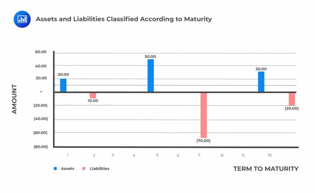Positive cash flows are received by the bank whenever assets expire, whereas when liabilities expire, the bank must pay negative cash flows.

Assuming further that the interest rate (yield) of the assets and liabilities is as shown below:

$$ \begin{array}{l|c|c} \textbf{Expiry} & \textbf{Assets} & \textbf{Liabilities} \\ \hline {1} & {5\%} & {0\%} \\ \hline {2} & {0\%} & {4\%} \\ \hline {3} & {0\%} & {0\%} \\ \hline {4} & {0\%} & {0\%} \\ \hline {5} & {6\%} & {0\%} \\ \hline {6} & {0\%} & {0\%} \\ \hline {7} & {0\%} & {0\%} \\ \hline {8} & {0\%} & {0\%} \\ \hline {9} & {0\%} & {0\%} \\ \hline {10} & {7\%} & {0\%} \\ \hline {> 10} & {0\%} & {0\%} \end{array} $$

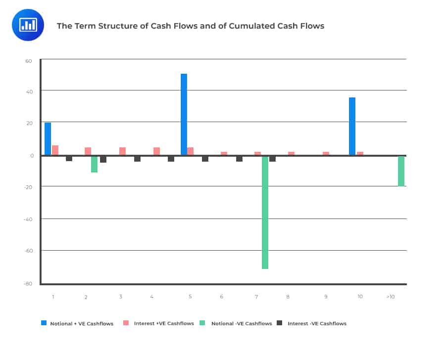
We can calculate the term structure of cash flows and cumulated cash flows, as shown in the table below:

$$ \textbf{Assets and Liabilities Reclassified According to Maturity} $$

$$ \begin{array}{l|c|c|c|c|c} \textbf{Expiry} & \textbf{Notional} & \textbf{Interest} & \textbf{Notional} & \textbf{Interest} & \textbf{TSECCF} \\ \hline \bf{1} & {20} & {6} & {0} & {-4} & {22} \\ \hline \bf{2} & {0} & {5} & {-10} & {-4} & {14} \\ \hline \bf{3} & {0} & {5} & {0} & {-3} & {16} \\ \hline \bf{4} & {0} & {5} & {0} & {-3} & {17} \\ \hline \bf{5} & {50} & {5} & {0} & {-3} & {69} \\ \hline \bf{6} & {0} & 2 & 0 & -3 & 68 \\ \hline \bf{7} & 0 & 2 & -70 & -3 & -3 \\ \hline \bf{8} & 0 & 2 & 0 & 0 & -2 \\ \hline \bf{9} & 0 & 2 & 0 & 0 & 0 \\ \hline \bf{10} & 30 & 2 & 0 & 0 & 32 \\ \hline \bf{> 10} & {0} & {-} & {-20} & {0} & {12} \\ \end{array} $$

Note that we use the ordinary method given as

$$ \text{TSECCF} (\text t_0, \text t_{\text k}) = \left\{ \text {CF}(\text t_0, \text t_0, \text t_1), {\text {CF}}(\text t_0, \text t_0, \text t_2),…, {\text {CF}}(\text t_0,\text t_0, \text t_{\text k})\right\} $$

A graphical representation is as shown:

Additionally, the cash flows of the TSECF are those produced by all the causes of cash flows. It hence means that the TSECF:

• Includes the cash flows from all current contracts that include the assets and liabilities. Cash flows are stochastic in many cases because they link to market variables, such as Libor or Euribor fixings.
• Cash flows in TSECF are adjusted to consider credit risks, and therefore credit models must be used to include defaults on an accumulative basis by also considering the correlation existing amongst the bank’s counterparties.
• Cash flows are adjusted to include liquidity options, and hence behavioral models are used for typical banking products such as sight deposits, credit link usage, and prepayment of mortgages.
• Cash flows originated by new business increasing the assets are included; they are typically stochastic in both the amount and time dimensions, so they are treated employing models that consider all related risks.
• The rollover of maturing liabilities by similar or different contracts, and new bond issuances (which could also be included in the new business category) to fund the increase in assets, are included.

Both the TSECF and the TSECCF do not include the flows produced by the sources of cash flows. The sources of cash flows are apparatus to manage the liquidity risk originated by the causes of cash flows.

Liquidity Generation Capacity

Liquidity generation capacity is the ability of a bank to generate positive cash flows, beyond contractual ones, from the sources of liquidity available on the balance sheet and off the balance sheet at a given date.

Ways in which LGC manifests itself:

1. Balance sheet expansion: from secured or unsecured funding; or

2. Balance sheet shrinkage: which results from selling assets.

When aiming to expand a balance sheet, we consider the following factors:

• Borrowing through an increase of deposits, typically in the interbank market (retail or wholesale unsecured funding);
• Withdrawal of credit lines the financial institution has received from other financial counterparties (wholesale unsecured funding); and/or
• Issuance of new bonds such as wholesale and retail unsecured funding.

A similar classification within LGC depends on the link between the generation of liquidity and the assets on the balance sheet so that we have:

1. Security-linked liquidity: the inclusion of secured withdrawals of credit lines received from other financial institutions, secured debt issuance, and selling of assets and repo; and
2. Security-unlinked liquidity: the inclusion of unsecured borrowing from new clients through new deposits, withdrawals of credit lines received from other financial institutions and, the unsecured bond issuance.

The security-linked liquidity is a bit more than the balance sheet liquidity (BSL) liquidity, or the liquidity obtained by balance sheet reduction.

The Term Structure of Liquidity Generation Capacity (TSLGC)

The TSLGC is the collection, a reference time \(\text t_0\), of liquidity that can be generated at a given time \(\text t_{\text i}\), by the sources of liquidity, up to an ending time \(\text t_{\text k}\) referred to as a terminal time expressed as follows:

$$ \begin{align*} & \text{TSLGC} ({\text t}_0,{\text t}_{\text k}) \\ & = \left\{ \text{AS} ({\text t_0,\text t_1}),{\text {RP}} ({\text t_0,\text t_1}),\text{USF}({\text t_0,\text t_1}),…,\text{AS}({\text t}_0,{\text t}_{\text k}),\text{RP}({\text t}_0,{\text t}_{\text k}),\text{USF}({\text t}_0,{\text t}_{\text k}) \right\}. \\ \end{align*} $$

In the equation, \(\text{AS} ({\text t_0,\text t_1})\) is the liquidity that can be generated by the sale of assets at the time \(\text t_{\text i}\), computed at the reference time \(\text t_0\). Similarly, \({\text {RP}} ({\text t_0,\text t_1})\) refers to secured funding (repurchase agreements, or repos) and \(\text{USF}({\text t_0,\text t_1})\) refers to unsecured funding.

The Term Structure of Cumulated Liquidity Generation Capacity (TSCLGC)

The term structure of cumulated LGC is the collection, at the reference time \(\text t_0\), of the cumulated liquidity generated at a time \(\text t_{\text i}\) up to a terminal time \(\text t_{\text k}\), using the sources of liquidity.

$$ \begin{align*} & \text{TSCLGC} ({\text t}_0,{\text t}_{\text k}) ={\sum_{\text i=0}^1 \text {TSLGC}({\text t}_0,{\text t}_{\text i}),\sum_{\text i=0}^2 \text{TSLGC}({\text t}_0,{\text t}_{\text i}),.,\sum_{\text i=0}^{\text k} \text{TSLGC}({\text t}_0,{\text t}_{\text k})}. \end{align*} $$

The sources of liquidity contributing to the TSLGC belong either to the banking or the trading book.

The Term Structure of Available Assets

At the end of the loan or repo, cash flows produced by a bond are typically given back to the borrower by the counterparty, although the contract may sometimes provide for various solutions. When an asset, such as a bond, is purchased by a bank, a corresponding outflow equivalent to the price is recorded in the cash position of the bank. All cash flows should be considered contract-related and included in the TSECF and the TSECCF. The possibility of the issuer defaulting is considered.

Transactions such as purchases, repo transactions, reverse repo transactions, sell/buyback transactions, and security lending affects cash flows and liquidity generation capacity, as discussed below.

Repo Transactions

During the repo agreements, the payments on the asset belong to the bank as it is the owner. Therefore, TSECF and TSECCF are not affected in any way. The TSAA of the asset is reduced by an amount equal to the notional of the repo agreement, whereas the cash flow received by the bank at the start and the negative cash flow at the end are both entered in the TSLGC. Repo transactions are viewed as liabilities on the balance sheet for the bank

Reverse Repo Transactions

In a reverse repo, the payments produced by the asset are not included in TSECF or the TSECCF as they don’t belong to the bank. However, we include the cash flow paid by the bank at the start and the cash flow received at the end of the contract, but only once. The TSAA of the asset is increased by an amount equal to the notional of the repo agreement while the TSLGC is not affected. Reverse repo transactions are viewed as assets on the balance sheet since they are collateralizable loans to the counterparty.

Sell/Buyback Transactions

In this transaction, the cash flows between the start and end of the contract should be taken from the TSECF and the TSECCF. Furthermore, the TSAA of the asset decreases by an amount equal to the notional of the sell/buyback contract. The TSLGC is affected in the same way as in the repo agreement since sell/buyback transactions are ways of generating balance sheet liquidity (BSL). Sell/buyback transactions represent a commitment to the bank at the end of the contract.

Buy/Sell-Back Transactions

In this transaction, the payments received for the asset before the sell-back belong to the bank so that they enter the TSECF and the TSECCF, along with the cash flows at the start and end that relate to the purchase and sale, since they are contract flows. The TSAA of the asset is increased by an amount equal to the notional of the buy/sell-back agreement. TSLGC is not affected, but the asset can be repoed until the end so that it can be altered until this date. Buy/sell back transactions represent an asset for the period of the contract.

Security Lending

In the security lending, both the payments received for the asset before the end of the contract and the interest paid by the counterparty at expiry belong to the bank, and they enter the TSECF and the TSECCF. The TSAA of the asset decreases by an amount equal to the notional of the lending since the bank cannot use it as collateral or sell it. The TSLGC is not affected, and the asset cannot produce any liquidity until the end of the contract. The transaction represents an asset on the bank’s balance sheet for the period of the contract.

Security Borrowing

In this transaction, the TSECF and the TSECCF are not affected besides the interest paid by the bank at the expiry of the borrowing. The TSAA of the asset increases by an amount equal to the notional of the borrowing since the bank can use it as collateral if it returns it to the counterparty at expiry. The TSLGC is not affected, but the asset can produce liquidity until the end of the contract. The transaction represents a liability of the bank.

Assets such as stocks have no definite expiry date. In this case, contract cash flows entering the TSECF and the TSECCF is simply the initial outflow representing the price paid to purchase the asset and the periodic dividend received. Note that TSLGC is continuously affected either because the contract is dealt to generate balance sheet liquidity (BSL) or because Liquidity generation capacity (LGC) is possibly increased over its lifetime. The only contract that does not increase the TSLGC is security lending, which decreases LGC related to BSL.

Practice Question

Which of the following statements correctly defines deterministic and stochastic cash flows?

A. Deterministic cash flows are those that can be predicted with certainty based on previous data, while stochastic cash flows vary randomly and are unpredictable.

B. Deterministic cash flows depend on various unpredictable factors, while stochastic cash flows are fixed and don’t change over time.

C. Deterministic cash flows are the revenues expected from the sale of a new product, while stochastic cash flows are the costs associated with setting up a new facility.

D. Deterministic cash flows are those affected by global economic conditions, while stochastic cash flows are those unaffected by external factors.

Solution

The correct answer is A.

Deterministic cash flows are those which can be predicted with certainty, as they don’t vary over time or with external factors. For instance, the cost of building a manufacturing facility which is already determined and contracted. On the other hand, stochastic cash flows are random and unpredictable, often influenced by various unpredictable factors. An example is the potential revenues from a new product in a volatile market.

B is incorrect. This statement gets the definitions reversed. Deterministic cash flows are those that are fixed and don’t change over time, while stochastic cash flows depend on various unpredictable factors.

C is incorrect. While the examples given might sometimes be true in certain contexts, they are not universally defining features of deterministic and stochastic cash flows. The definition should not be based solely on examples but on the nature of the cash flows themselves.

D is incorrect. Global economic conditions can affect both deterministic and stochastic cash flows. The distinguishing factor between them isn’t whether they are affected by external factors, but the predictability and variability of the cash flows.

Things to Remember

• Deterministic cash flows provide a predictable financial outlook, facilitating confident business and strategic planning.
• Stochastic cash flows arise in more dynamic environments, where factors such as market volatility can introduce variations.
• Deterministic models simplify complex real-world situations, allowing for clear decision-making. However, they might not always capture the full scope of potential outcomes.
• Stochastic models can cater to a wider range of possibilities, making them valuable in unpredictable markets or sectors, albeit at the cost of complexity.