Are you preparing for the FRM Part 1 exam? Whether you’re on your daily commute, taking a break at work, or winding down at home, AnalystPrep’s FRM Part 1 Study Notes make it easy to revise on the go—without carrying heavy textbooks.

Our study notes are structured chapter-by-chapter, reflecting the learning objectives outlined in GARP’s official curriculum. Not a single key concept is left out. We’ve condensed the most important exam material into clear, easy-to-digest summaries, so you can:

✔ Save Time – Get straight to the essential concepts without sifting through excessive details.
✔ Understand Quickly – Simple explanations help you grasp quantitative finance, risk management, and investment topics effortlessly.
✔ Revise Anywhere – Study at home, in the office, or even on the subway to work.

If you’re new to the FRM exam, our notes help you build a strong foundation in risk management, ensuring you cover all 104 readings in a structured way.
Also, if you’re retaking the exam, use our study guides to pinpoint your weak areas and reinforce core concepts—without wasting time on unnecessary details.

Absorbing the FRM curriculum is no easy feat, but we make it manageable. Our comprehensive, exam-oriented approach ensures you retain key information efficiently and confidently walk into exam day prepared.

After completing this reading, you should be able to:

• Explain how to test whether regression is affected by heteroskedasticity.
• Describe approaches to using heteroskedastic data.
• Characterize multicollinearity and its consequences; distinguish between multicollinearity and perfect collinearity.
• Describe the consequences of excluding a relevant explanatory variable from a model and contrast those with the consequences of including an irrelevant regressor.
• Explain two model selection procedures and how these relate to the bias-variance tradeoff.
• Describe the various methods of visualizing residuals and their relative strengths.
• Describe methods for identifying outliers and their impact.
• Determine the conditions under which OLS is the best linear unbiased estimator.

Regression Model Specifications

Model specification is a process of determining which independent variables should be included in or excluded from a regression model.

That is, an ideal regression model should consist of all the variables that explain the dependent variables and remove those that do not.

Model specification includes the residual diagnostics and the statistical tests on the assumptions of OLS estimators. Basically, the choice of variables to be included in a model depends on the bias-variance tradeoff. For instance, large models that include the relevant number of variables are likely to have unbiased coefficients. On the other side, smaller models lead to accurate estimates of the impact of removing some variables.

The conventional specification makes sure that the functional form of the model is adequate, the parameters are constant, and the homoscedasticity assumption is met.

The Omitted Variables

An omitted variable is one with a non-zero coefficient, but they are excluded in the regression model.

Effects of Omitting Variables

1. The remaining variables sustain the impact of the excluded variables in terms of the common variation. Thus, they do not consistently approximate the change in the independent variable on the dependent variable while keeping all other things constant.
2. The magnitude of the estimated residuals is larger than the true value. This is true since the estimated residuals have the true value and the effect of the omitted value that cannot be reflected in the included variables.

Illustration of the Omitted Variables

Suppose that the regression model is stated as:

$$ {\text Y}_{\text i}=\alpha+\beta_{\text i} {\text X}_{1{\text i}}+\beta_2 {\text X}_{2{\text i}}+\epsilon_{\text i} $$

If we omit \({\text X}_{2}\) from the estimated model, then the model is given by:

$$ {\text Y}_{\text i}=\alpha+\beta_{\text i} {\text X}_{1{\text i}}+\epsilon_{\text i} $$

Now, in large samples sizes, the OLS estimator \({\hat \beta}_1\) converges to:

$$ \beta_1+\beta_2 \delta $$

Where:

$$ \delta=\frac {{\text {Cov}}({\text X}_1,{\text X}_2)}{{\text {Var}}({\text X}_1)} $$

\(\delta\) is the population slope coefficient in a regression of \({\text X}_2\) on \({\text X}_1\).

It is clear that the bias – due to the omitted variable – depends on the population coefficient of the excluded variable \(\beta_2\) and the relational strength of the \({\text X}_2\) and \({\text X}_1\), represented by \(\delta\).

When the correlation between \({\text X}_1\) and \({\text X}_2\) is high, \({\text X}_1\) can explain a significant proportion of variation in \({\text X}_2\) and hence the bias is high. On the other hand, if the independent variables are uncorrelated, that is \(\delta=0\) then \(\hat \beta_1\) is a consistent estimator of \(\beta_1\).

Conclusively, the omitted variable leads to biasness of the coefficient on the variables that are correlated with the omitted variables.

Inclusion of Extraneous Variables

An extraneous variable is one that is unnecessarily included in the model, whose actual coefficient is 0 and is consistently estimated to be 0 in large samples. If we include these variables is costly.

Illustration of Effect of Inclusion of Extraneous Random Variables

Recall that the adjusted \({\text R}^2\) is given by:

$$ {{\bar {\text R}}^2}=1-\xi {\frac {\text {RSS}}{\text {TSS}}} $$

Where:

$$ \xi=\frac {({\text n}-1)}{({\text n}-{\text k}-1)} $$

Looking at the formula above, adding more variables increase the value of k which in turn increases the value of \(\xi\) and hence reducing the value of \({{\bar {\text R}}^2}\). However, if the model is large, then RSS is smaller which reduces the effect of \(\xi\) and produces larger \({{\bar {\text R}}^2}\).

Contrastingly, this is not always the case when the true coefficient is equal to 0 because, in this case, RSS remains constant as \(\xi\) increases leading to a smaller \({{\bar {\text R}}^2}\) and a large standard error.

Lastly, if the correlation between \({\text X}_1\) and \({\text X}_2\) increases, the standard error value rises.

The Bias-Variance Tradeoff

The bias-variance tradeoff amounts to choosing between including irrelevant variables and excluding relevant variables. Bigger models tend to have a low bias level because it includes more relevant variables. However, they are less accurate in approximating the regression parameters due to the possibility of involving extraneous variables.

Moreover, regression models with fewer independent variables are characterized by low estimation error but are more prone to biased parameter estimates.

Methods of Choosing a Model from a Set of Independent Variables

1. General-to-Specific Model SelectionIn the general-to-specific method, we start with a large general model that incorporates all the relevant variables. Then, the reduction of the general model starts. We use hypothesis tests to establish if there are any statistically insignificant coefficients in the estimated model.  When such coefficients are found, the variable with the coefficient with the smallest t-statistic is removed. The model is then re-estimated using the remaining set of independent variables. Once more, hypothesis tests are carried out to establish if statistically insignificant coefficients are present. These two steps (remove and re-estimate) are repeated until all coefficients that are statistically insignificant have been removed.
2. m-fold Cross-ValidationThe m-fold cross-validation model-selection method aims at choosing the model that’s best at fitting observations not used to estimate parameters. How is this method executed? As a first step, the number of models has to be decided, and this is determined in part by the number of explanatory variables. When this number is small, the researcher can consider all the possible combinations. With 10 variables, for example, 1,024 (=) distinct models can be constructed.The cross-validation process proceeds as follows:
   1. Shuffle the dataset randomly.
   2. Split the dataset into m groups.
   3. Estimate parameters using m-1 of the groups; these groups make up the training block. The excluded group is referred to as the validation block.
   4. Use the estimated parameters and the data in the excluded block (validation block) to compute residual values. These residuals are referred to as out-of-sample residuals since they are arrived at using data not included in the sample used to develop the parameter estimates.
   5. Repeat parameter estimation and residual computation a total of m times; each group has to serve as the validation block and is used to compute residuals.
   6. Compute the sum of squared errors using the residuals estimated from the out-of-sample data.
   7. Select the model with the smallest out-of-sample sum of squared residuals.

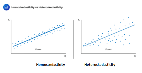
Heteroskedasticity

Recall that homoskedasticity is one of the critical assumptions in determining the distribution of the OLS estimator. That is, the variance of \(\epsilon_i\) is constant and that it does not vary with any of the independent variables; formally stated as \(\text{Var}(\epsilon_i│{\text X}_{1{\text i}},{\text X}_{2{\text i}},…,{\text X}_{k{\text i}} )=\delta^2\). Heteroskedasticity is a systematic pattern in the residuals where the variances of the residuals are not constant.

Test for Heteroskedasticity

Halbert White proposed a simple test with the following two-step procedures:

1. Approximate the model and calculate the residuals, \(\epsilon_{\text i}\)
2. Regress the squared residuals on:
   1. A constant
   2. All explanatory variables
   3. The cross product of all the independent variables, including the product of each variable with itself.

Consider an original model with two independent variables:

$$ {\text Y}_{\text i}=\alpha+\beta_{\text i} {\text X}_{1{\text i}}+\beta_2 {\text X}_{2{\text i}}+\epsilon_{\text i} $$

The first step is to calculate the residuals by utilizing the OLS parameter estimators:

$$ {\hat \epsilon}_{\text i}={\text Y}_{\text i}-{\hat {\alpha} }-{\hat {\beta}}_1 {\text X}_{1{\text i}}-{\hat \beta}_2 {\text X}_{2{\text i}} $$

Now, we need to regress the squared residuals on a constant \({\text X}_1,{\text X}_2,{\text X}_1^2,{\text X}_2^2\) and \({\text X}_1 {\text X}_2\)

$$ {\hat \epsilon}_{\text i}^2={\Upsilon}_0+{\Upsilon}_1 {\text X}_{1{\text i}}+{\Upsilon}_2 {\text X}_{2{\text i}}+{\Upsilon}_3 {\text X}_{1{\text i}}^2+{\Upsilon}_4 {\text X}_{2{\text i}}^2+{\Upsilon}_5 {\text X}_{1{\text i}}^2 {\text X}_{2{\text i}}^2 $$

If the data is homoscedastic, then \({\hat \epsilon}_{\text i}^2\) must not be explained by any of the variables and the null hypothesis is: \({\text H}_0:{\Upsilon}_1=⋯={\Upsilon}_5=0\)

The test statistic is calculated as \(\text {nR}^2\) where \({\text R}^2\) is calculated in the second regression and that the test statistic has a \(\chi_{ \frac{{\text k}{(\text k}+3)}{2} }^2\) (chi-distribution), where k is the number of explanatory variables in the first-step model.

For instance, if the number of explanatory variables is two, k=2, then the test statistic has a \(\chi_5\) distribution.

Modeling Heteroskedastic Data

The three common methods of handling data with heteroskedastic shocks include:

1. Ignoring the heteroskedasticity when approximating the parameters and utilizing the White covariance estimator in hypothesis tests. However simple, this method leads to less accurate model parameter estimates compared to other methods that address heteroskedasticity.
2. Transformation of data. For instance, positive data can be log-transformed to try and remove heteroskedasticity and give a better view of data. Another transformation can be in the form of dividing the dependent variable by another positive variable.
3. Use of weighted least squares (WLS).This is a complicated method that applies weights to the data before approximating the parameters. That is if we know that \(\text{Var}(\epsilon_{\text i} )={\text w}_{\text i}^2 \sigma^2\) where \({\text w}_{\text i}\) is known then we can transform the data by dividing by \({\text w}_{\text i}\) to remove the heteroskedasticity from the errors. In other words, the WLS regresses \(\frac {{\text Y}_{\text i}}{{\text w}_{\text i}}\) on \(\frac {{\text X}_{\text i}}{{\text w}_{\text i}}\) such as:$$ \begin{align*} \frac {{\text Y}_{\text i}}{{\text w}_{\text i}} & =\alpha \frac {1}{{\text w}_{\text i}} +\beta \frac {{\text X}_{\text i}}{{\text w}_{\text i}} +\frac {\epsilon_{\text i}}{{\text w}_{\text i}} \\ {\bar {\text Y}}_{\text i} & =\alpha {\bar {\text C} }_{\text i}+\beta {\bar {\text X} }_{\text i}+{\bar {\epsilon}}_{\text i} \\ \end{align*} $$

Note that the parameters of the model above are estimated using OLS on the transformed data. That is, the weighted version of \({\text Y}_{\text i}\) which is \({\bar {\text Y}}_{\text i} \) on two weighted explanatory variables \({\bar {\text C}}_{\text i}=\frac {1}{{\text w}_{\text i}}\) and \({\bar {\text X}}_{\text i}=\frac {{\text X}_{\text i}}{{\text w}_{\text i}}\) . Note that the WLS model does not clearly include the intercept \(\alpha\), but the interpretation is still the same, that is, the intercept.

Multicollinearity

Multicollinearity occurs when others can significantly explain one or more independent variables. For instance, in the case of two independent variables, there is evidence of multicollinearity if the \({\text R}^2\) is very high if one variable is regressed on the other.

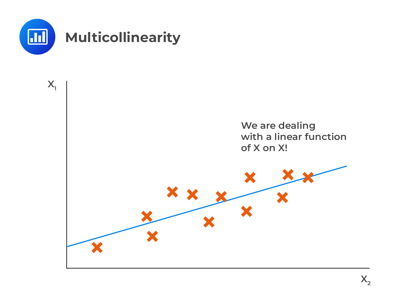In contrast with multicollinearity, perfect correlation is where one of the variables is perfectly correlated to others such that the \({\text R}^2\) of regression of \({\text X}_{\text j}\) on the remaining independent variable is precisely 1.

Conventionally, when \({\text R}^2\) is above 90% leads to problems in medium sample sizes such as that of 100. Multicollinearity does not pose an issue in parameter approximation, but rather, it brings some difficulties in modeling the data.

When multicollinearity is present, some of the coefficients in a regression model are jointly statistically significant (F-statistic is substantial), but the individual t-statistic is very small (less than 1.96) since the regression analysis assumes the collective effect of the variables rather than the individual effect of the variables.

Addressing Multicollinearity

There are two ways of dealing with multicollinearity:

1. Ignoring multicollinearity altogether since it is technically not a problem.
2. Identification of the multicollinear variables and excluding them from the model. Identification of multicollinear variables using the variance inflation factor which compares the variance of the regression coefficients on independent variable \({\text X}_{\text j}\) in two models: one that incorporates only \({\text X}_{\text j}\) and one that omits k independent variables: $$ {\text X}_{\text {ji}}=\Upsilon_0+\Upsilon_1 {\text X}_{1{\text i}}+⋯+\Upsilon_{{\text j}-1} X_{{\text j}-1{\text i}}+\Upsilon_{{\text j}+1} {\text X}_{{\text j}+1{\text i}}+⋯+\Upsilon_{\text k} {\text X}_{{\text k}{\text i}}+\eta_{\text i} $$The variance inflation factor (VIF) for the variable \({\text X}_{\text j}\) is given by:$$ \text{VIF}_{\text j}=\frac {1}{1-{\text R}_{\text j}^2 } $$Where \({\text R}_{\text j}^2\) originates from regressing \({\text X}_{\text j}\) on the other variable in the model. When the value of the VIF is above 10, then it is considered too much and the variable should be excluded from the model.

Residual Plots

Residual plots are utilized to identify the deficiencies in a model specification. When the residual plots are not systematically related to any of the included independent (explanatory variables) and are relatively small (within \(\pm\)4s, where s is the standard shock deviation of the model) in magnitude, then the model is ideally good.

Residual plot is a graph of \(\hat \epsilon_{\text i}\) (vertical axis) against the independent variables \({\text x}_{\text i}\). Alternatively, we could use the standardized residuals \(\frac {\hat \epsilon_{\text i}}{\text s}\) which makes sure that the deviation is apparent.

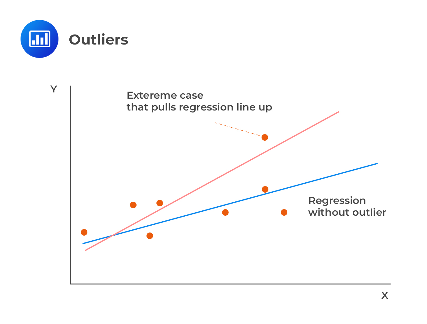
Outliers

Outliers are values that, if removed from the sample, produce large changes in the estimated coefficients. They can also be viewed as data points that deviate significantly from the normal objects as if a different mechanism generated them.

Cook’s distance helps us measure the impact of dropping a single observation j on a regression (and the line of best fit).

The Cook’s distance is given by:

$$ {\text D}_{\text j}=\frac {\sum_{\text i=1}^{\text n} \left( {{\bar {\text Y}}_{\text i}}^{(-{\text j})}-{\hat {\text Y} }_{\text i} \right)^2 }{\text{ks}^2 } $$

Where:

\({{\bar {\text Y}}_{\text i}}^{(-{\text j})}\)=fitted value of \({{\bar {\text Y}}_{\text i}}\) when the observed value j is excluded, and the model is approximated using n-1 observations.

k=number of coefficients in the regression model

\(\text s^2\)=estimated error variance from the model using all observations

When a variable is an inline (it does not affect the coefficient estimates when excluded), the value of its Cook’s distance (\({\text D}_{\text j}\)) is small. On the other hand, \({\text D}_{\text j}\) is higher than 1 if it is an outlier.

Example: Calculating Cook’s Distance

Consider the following data sets:

$$ \begin{array}{c|c|c} \textbf{Observation} & \textbf{Y} & \textbf{X} \\ \hline{1} & {3.67} & {1.85} \\ \hline {2} & {1.88} & {0.65} \\ \hline {3} & {1.35} & {-0.63} \\ \hline {4} & {0.34} & {1.24} \\ \hline {5} & {-0.89} & {-2.45} \\ \hline {6} & {1.95} & {0.76} \\ \hline {7} & {2.98} & {0.85} \\ \hline {8} & {1.65} & {0.28} \\ \hline {9} & {1.47} & {0.75} \\ \hline {10} & {1.58} & {-0.43} \\ \hline {11} & {0.66} & {1.14} \\ \hline {12} & {0.05} & {-1.79} \\ \hline {13} & {1.67} & {1.49} \\ \hline {14} & {-0.14} & {-0.64} \\ \hline {15} & {9.05} & {1.87} \\ \end{array} $$

If you look at the data sets above, it is easy to see that observation 15 is more significant than the rest of the observations, and there is a possibility of an outlier. However, we need to ascertain this.

We begin by fitting the whole dataset (\({{\bar {\text Y}}_{\text i}}\)) and then the 14 observations which remain after excluding the dataset that we believe is an outlier.

If we fit the whole dataset, we get the following regression equation:

$$ {{\bar {\text Y}}_{\text i}}=1.4465+1.1281{\text X_{\text i}} $$

And if we exclude the observation that we believe it is an outlier we get:

$$ {{\bar {\text Y}}_{\text i}}^{(-{\text j})}=1.1516+0.6828{\text X_{\text i}} $$

Now the fitted values are as shown below:

$$ \begin{array}{c|c|c} \textbf{Observation} & \textbf{Y} & \textbf{X} & \bf{{{\bar {\text Y}}_{\text i}}} & \bf{{{\bar {\text Y}}_{\text i}}^{(-{\text j})}} & \bf{\left({{\bar {\text Y}}_{\text i}}^{(-{\text j})}-{{{\bar {\text Y}}_{\text i}}} \right)^2} \\ \hline {1} & {3.67} & {1.85} & {3.533} & {2.4148} & {1.2504} \\ \hline {2} & {1.88} & {0.65} & {2.179} & {1.5954} & {0.3406} \\ \hline {3} & {1.35} & {0.63} & {0.7358} & {0.7214} & {0.0002} \\ \hline {4} & {0.34} & {1.24} & {2.8453} & {1.9983} & {0.7174} \\ \hline {5} & {0.89} & {2.45} & {-1.3174} & {-0.5213} & {0.6338} \\ \hline {6} & {1.95} & {0.76} & {2.3039} & {1.6705} & {0.4012} \\ \hline {7} & {2.98} & {0.85} & {2.4053} & {1.732} & {0.4533} \\ \hline {8} & {1.65} & {0.28} & {1.7624} & {1.3428} & {0.1761} \\ \hline {9} & {1.47} & {0.75} & {2.2926} & {1.6637} & {0.3955} \\ \hline {10} & {1.58} & {0.43} & {0.9614} & {0.858} & {0.0107} \\ \hline {11} & {0.66} & {1.14} & {2.7325} & {1.921} & {0.6585} \\ \hline {12} & {0.05} & {1.79} & {-0.5728} & {-0.07061} & {0.2522} \\ \hline {13} & {1.67} & {1.49} & {3.1274} & {2.169} & {0.9185} \\ \hline {14} & {0.14} & {0.64} & {0.7245} & {0.7146} & {0.0001} \\ \hline {15} & {9.05} & {1.87} & {3.556} & {2.4284} & {1.2715} \\ \hline {} & {} & {} & {} & \textbf{Sum} & \bf{7.4800} \\ \end{array} $$

If the \(\text s^2=3.554\) the Cook’s distance is given by:

$$ {\text D}_{\text j}=\frac {\sum_{\text i=1}^{\text n} \left( {{\bar {\text Y}}_{\text i}}^{(-{\text j})}-{\hat {\text Y} }_{\text i} \right)^2 }{\text{ks}^2 } =\frac {7.4800}{2×3.554}=1.0523 $$

Since \({\text D}_{\text j} > 1\), then observation 15 can be considered as an outlier.

Strengths of Ordinary Least Squares (OLS )

OLS  is the Best Linear Unbiased Estimator (BLUE) when some key assumptions are met, which implies that it can assume the smallest possible variance among any given estimator that is linear and unbiased:

• Linearity: the parameters being estimated using the OLS method must be themselves linear.
• Random: the data must have been randomly sampled from the population.
• Non-Collinearity: the regressors being calculated should not be perfectly correlated with each other.
• Exogeneity: the regressors aren’t correlated with the error term.
• Homoscedasticity: the variance of the error term is constant

However, being a BLUE estimator comes with the following limitations:

1. A big proportion of the estimators are not linear such as maximum likelihood estimators (but biased).
2. BLUE property is heavily dependent on residuals being homoskedastic. In the case that the variances of residuals vary the independent variables, then it is possible to construct linear unbiased estimators (LUE) of the coefficients α and β using WLS but with extra assumptions.

When the residuals and iid and normally distributed with a mean of 0 and variance of \(\sigma^2\), formally stated as \(\epsilon_{i} \sim^{iid} {\text N}(0,\sigma^2)\) makes the upgrades BLUE to BUE (Best Unbiased Estimator) by virtue having the smallest variance among all linear and non-linear estimators. However, errors being normally distributed is not a requirement for accurate estimates of the model coefficients or a necessity for desirable properties of estimators.

Practice Question 1

Which of the following statements is/are correct?

I. Homoskedasticity means that the variance of the error terms is constant for all independent variables.

II. Heteroskedasticity means that the variance of error terms varies over the sample.

III. The presence of conditional heteroskedasticity reduces the standard error.

1. Only I
2. II and III
3. All statements are correct
4. None of the statements are correct

Solution

The correct answer is C.

All statements are correct.

If the variance of the residuals is constant across all observations in the sample, the regression is said to be homoskedastic. When the opposite is true, the regression is said to exhibit heteroskedasticity, i.e., the variance of the residuals is not the same across all observations in the sample. The presence of conditional heteroskedasticity poses a significant problem: it introduces a bias into the estimators of the standard error of the regression coefficients. As such, it understates the standard error.

Practice Question 2

A financial analyst fails to include a variable that inherently has a non-zero coefficient in his regression analysis. Moreover, the ignored variable is highly correlated with the remaining variables.

What is the most likely deficiency of the analyst’s model?

1. Omitted variable bias.
2. Bias due to the inclusion of extraneous variables.
3. Presence of heteroskedasticity.
4. None of the above.

Solution

The correct answer is A.

Omitted variable bias occurs under two conditions:

I. A variable with a non-zero coefficient is omitted

II. A omitted variable is correlated with remaining (included) variables.

These conditions are met in the description of the analyst’s model.

Option B is incorrect since an extraneous variable is one that is unnecessarily included in the model, whose true coefficient and consistently approximated value is 0 in large sample sizes.

Option C is incorrect because heteroskedasticity is a condition where the variance of the errors varies systematically with the model’s independent variables.