Breakeven Analysis

Companies can be grouped as operating in perfect or imperfect competitive environments depending on the slope of the demand curve.

Perfectly Competitive Environment

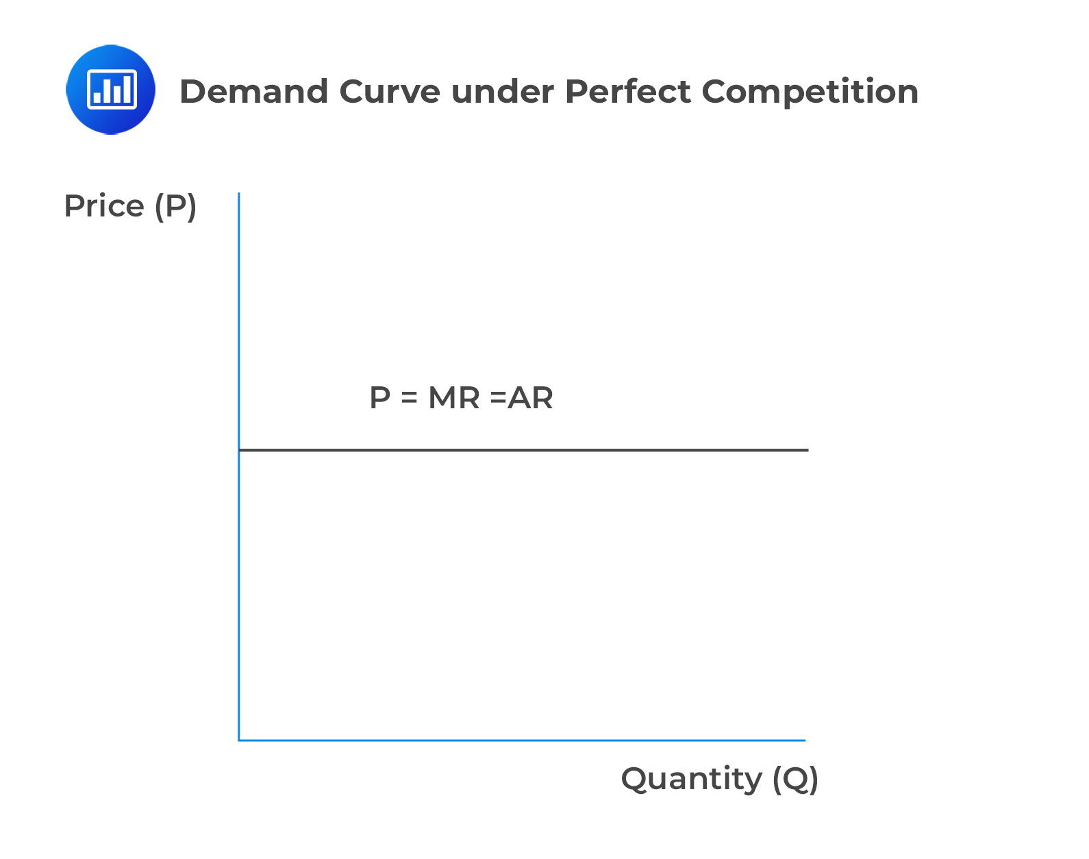
In a perfectly competitive environment, firms are the price takers. That is, it must the market price of its output so that its demand curve is perfectly elastic and horizontal.

In a perfectly competitive environment, marginal revenue (MR) is equal to the price per unit output (P). Moreover, the average revenue (AR) is also equal to the price per unit. Put simply, \(P = MR= AR\)

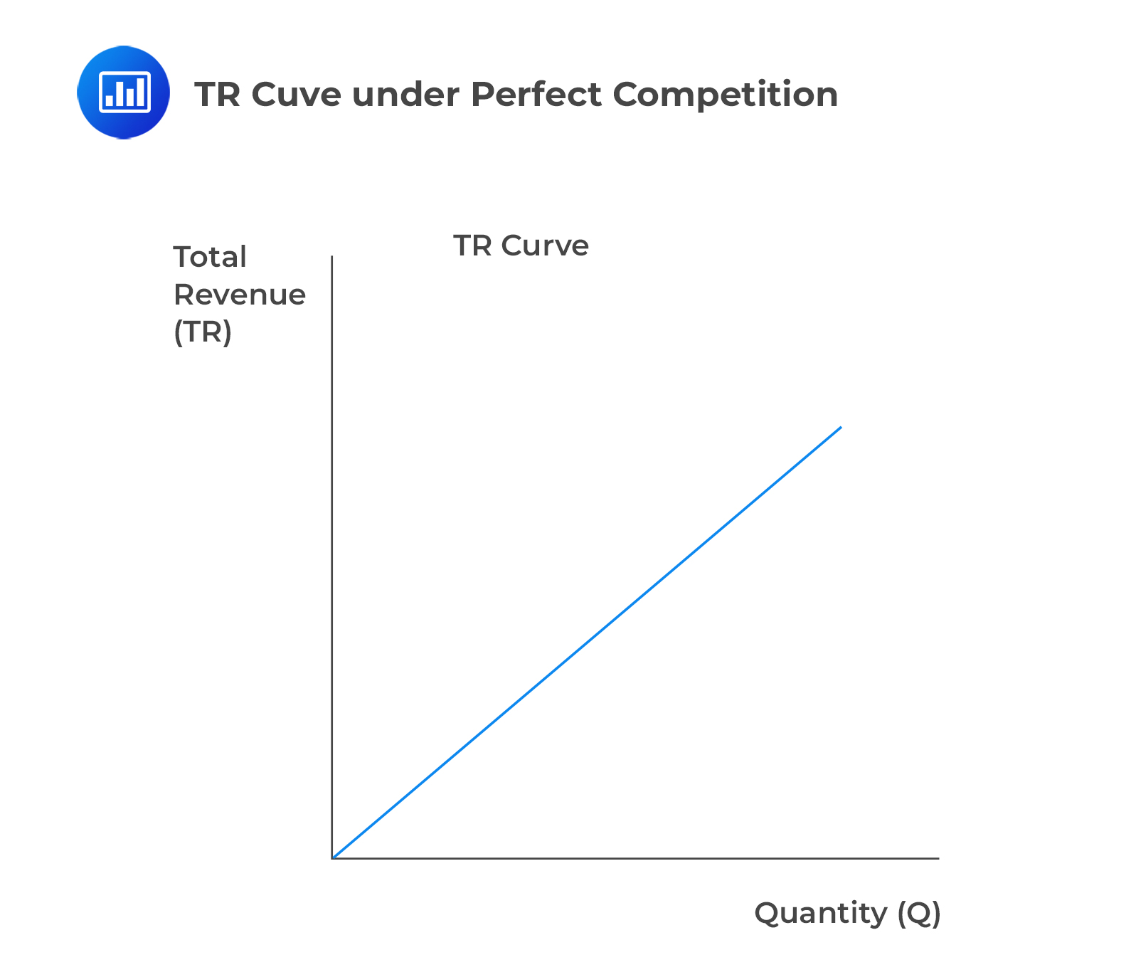
In perfect competition, total revenue (TR) is equal to price times quantity. That is, TR = (P)(Q). However, note that in perfect competition, the market determines the price. As such, when a company sells an additional unit, TR rises by an amount equal to the price per unit (P). Consider the following graph:

Imperfectly Competitive Environment

In the case of imperfect competition, the demand curve has a negative slope.

Assume that a company is monopolistic. In this case, the firm has control over the price. Simply stated, the price is a function of the quantity. Mathematically, this is stated as:

$$ P=f(Q) $$

As such, the total revenue (TR) is given by:

$$ TR = f(Q)\times Q $$

Assuming that the demand curve is linear and negatively sloped, TR is equal to the total expenditure of all the buyers in the market.

Note that a monopolist sets the price. As such, when the price decreases, the quantity sold increases. This initially increases the total expenditure by the buyers and, hence, the TR of the company because a price decrease is overpowered by the increase in units sold. This happens in the range where MR is positive, and demand is elastic. Consider the following image:

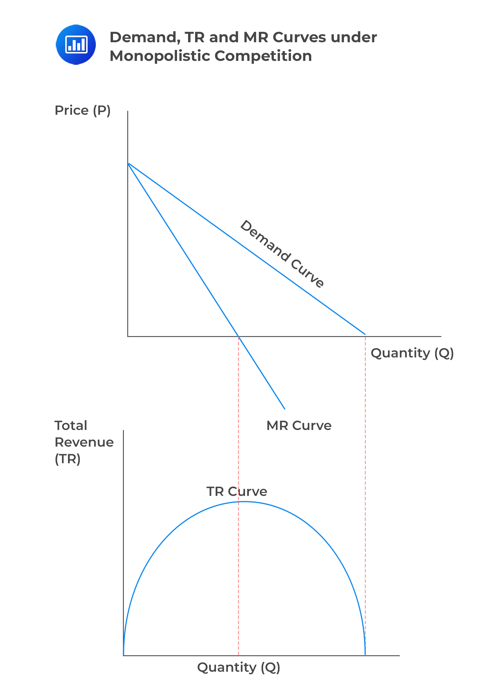
When the price drops, even though more units are sold, the total spending by buyers decreases because the price reduction has a greater impact. This happens when marginal revenue (MR) is negative and demand is inelastic.

Profit-Maximization, Breakeven, and Shutdown Points of Production

We use the short-run total cost (STC) curves and its associated TR curves to show the profit maximization point. The short-term run and long run time for a company depends on the ability of the firm to adjust the amounts of the fixed resources it utilizes.

The short run is the amount of time during which at least one of the factors of production, such as technology, physical capital, and plant size, is fixed. On the other hand, the long run is the time period during which all factors of production are variable. Moreover, in the long run, companies can enter or exit the market depending on the profitability analysis.

The long run is also termed the planning horizon because the company can choose the short-run position or optimal operating size that maximizes profit. Specifically, a company always operates in the short run and plans in the long run.

Profit-Maximization Point

Under Perfect Competition

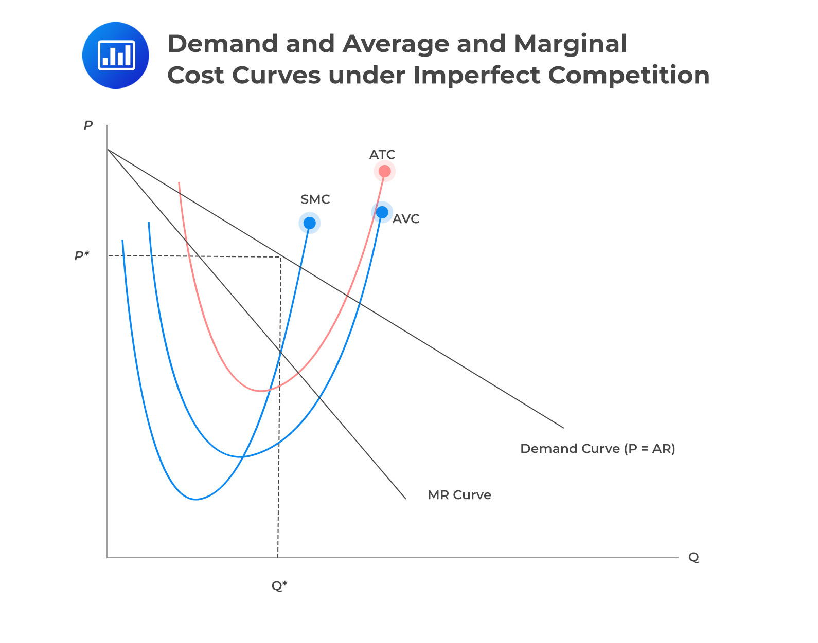
Consider the following demand and average and marginal cost curves for the firm under conditions of perfect competition:

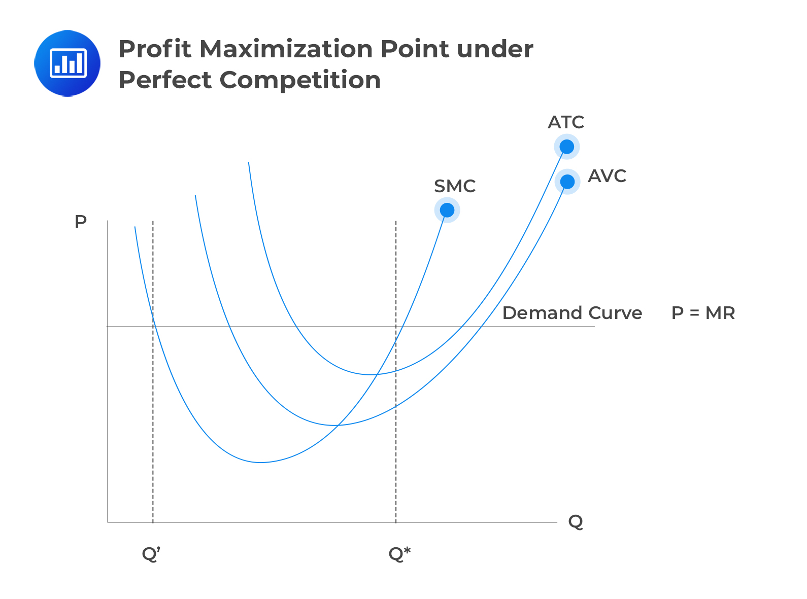
The company maximizes its profit by producing at an output level of \(Q^\ast\), where the price matches the short-run marginal cost (SMC) and the SMC is increasing. However, at a different output, denoted as Q’, even though the price is equivalent to the SMC, the SMC has not yet started to increase but is still decreasing. Hence, this cannot be a point where profit is maximized.

If the market price were to increase, the company’s demand and marginal revenue (MR) curve would shift upwards, leading the firm to determine a new optimal production output greater than \(Q^\ast\). On the contrary, if the market price decreased, the demand and MR curve would move downward, setting a decreased profit–maximizing output.

As shown in the image, this company is realizing positive economic profits since the market price is greater than the average total cost (ATC) when producing at \(Q^\ast\). This kind of profit is achievable in the short run. However, in the long run, rival companies would likely enter the market aiming to obtain some of these profits, subsequently pushing the market price down to match each company’s ATC.

Under Imperfect Competition

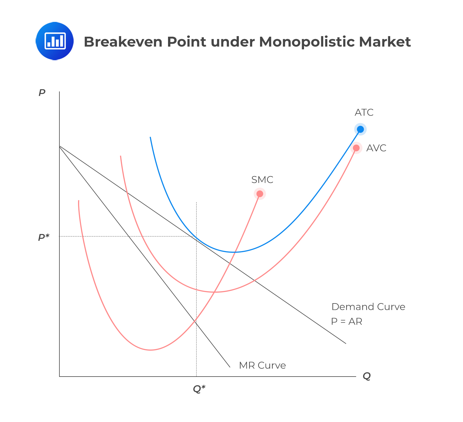
Consider the following demand and average and marginal cost curves for the firm under imperfect competition (monopolist) conditions.

The marginal revenue (MR) and demand curves for a monopolist are not the same. However, the rule for maximizing profits remains consistent: Identify the quantity (Q) where short-term marginal cost (SMC) equals MR, which in this instance is at \(Q^\ast\).

After determining the suitable output level, the best price to set is indicated by the firm’s demand curve at price \(P^\ast\). The monopolistic company enjoys a positive economic profit since its price is higher than its average total cost (ATC).

The entry barriers, which grant the firm its monopolistic dominance, ensure that potential competitors cannot erode the firm’s profit margins.

Breakeven Analysis

A firm reaches its breakeven point when its total revenue (TR) matches its total cost (TC). Similarly, a firm is at the breakeven point when its average revenue (AR) is precisely equal to its average total cost (ATC). This holds true in both perfect and imperfect competitive environments.

While management usually aims for maximum profits, some firms can only cover all their economic costs. Economic costs include both accounting and implicit opportunity costs.

When the firm’s revenue is equal to its economic costs, it implies that the company can cover the opportunity cost of all factors of production. In this case, the firm is said to be earning normal profit but not positive economic profit.

Firms operating in a perfectly competitive environment will not be able to earn a positive economic profit in the long run because an excess rate of return will lure new entrants into the market. These newcomers would increase the supply, subsequently pushing the market price down until every firm merely achieves a normal profit. It’s crucial to understand that this scenario doesn’t mean the firm is making zero accounting profit.

Consider the following graph of a firm under perfect competition:

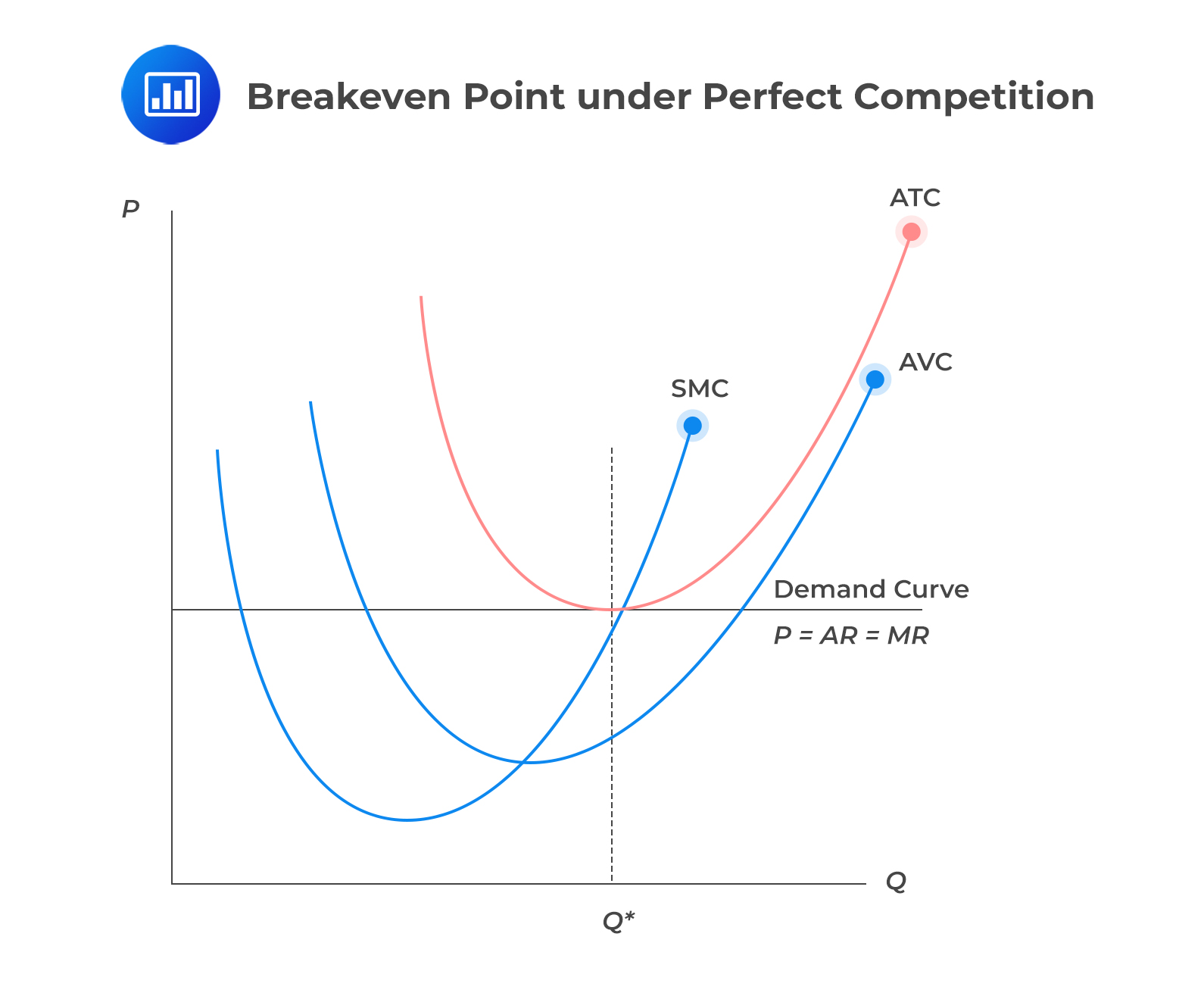
Recall that the best a firm can do is to break even. Note that in the graph above, the level of output where SMC = MR is where P = ATC. This implies that economic profit is zero, and the firm is at a breakeven point.

The equivalent graph of a monopolist firm is shown below:

Shutdown Analysis

In the long run, if a firm can’t make zero economic profit, it will shut down as it can’t cover all its costs, including labor and capital. But in the short run, a firm might keep operating even if it doesn’t make zero economic profit.

Recall that fixed costs are expenses that remain constant regardless of a company’s production level, such as rent and fixed interest charges. On the other hand, variable costs are directly tied to the volume of production and include items like raw materials, wages, and other costs that vary based on production levels.

As long as the firm’s revenues cover its variable costs, it can continue operations, covering both variable and a portion of its fixed costs (essentially operating at a loss). This is possible if the price (P) per unit is greater than the average variable cost (AVC).

However, in the long run, the firm should exit the industry if market prices do not increase, as it becomes unsustainable to stay in the market without the potential for higher returns.

When deciding whether to continue operating in the short run, it is essential to disregard sunk costs since they have already been incurred and are irrecoverable, regardless of the firm’s choice.

This is shown in the graph below:

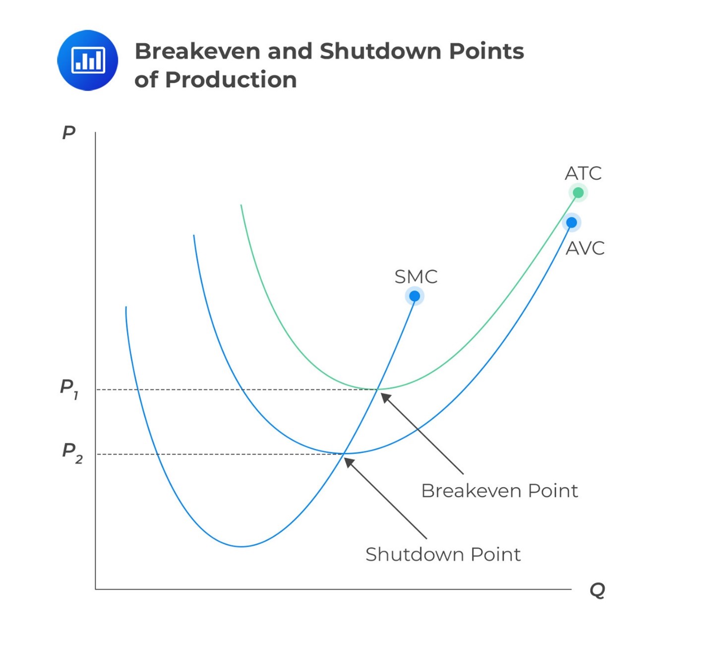
When the price is higher than \(P_1\), the firm has the potential to achieve a positive profit, and it definitely should remain in operation. If the price falls below \(P_2\), which represents the lowest average variable cost (AVC), the firm will fail to cover its variable expenses, and it should cease operations.

For prices ranging between P2 and P1, it’s beneficial for the firm to keep operating in the short term because it can meet all variable costs and contribute to covering the fixed costs.

The lowest point on the AVC curve is the shutdown point, and the lowest point on the average total cost (ATC) is the breakeven point.

The following table shows the conditions for a firm to operate, shut down, or exit the market in the short and long run.

$$ \begin{array}{l|l|l}
{\textbf{Relationship between} \\ \textbf{Revenue and Costs}} & \textbf{Short-Term Decision} & \textbf{Long-Run-Decision} \\ \hline
{\text{Total cost = Total} \\ \text{revenue} } & \text{Remain in the market} & \text{Remain in the market} \\ \hline
{ \text{Total revenue < Total} \\ \text{costs and > Total} \\ \text{variable costs}} & \text{Remain in the market} & \text{Leave the market} \\ \hline
{ \text{Total revenue < Total} \\ \text{variable cost}} & \text{Cease production} & { \text{Continue operating in} \\ \text{the market} }
\end{array} $$

Example: Shut-down Point of Production

Assume that a manufacturing company produces 1000 units and sells them at $5 each (Total Revenue (TR) is 5 \(\times\) 1,000=$5,000), Average Total Cost (ATC) is $7,000, fixed cost (FC) is $4000, and a variable cost (VC) is $3,000 for all units.

Evidently, this manufacturing company is operating at a loss of -$2000 (economic loss). In economics, we assume that the FC cannot be avoided. The company is obliged to pay it up regardless of whether it operates or not. That is, if it closes its operations, the revenue will be zero, but it will still incur a $4,000 fixed cost.

If it continues its operations, it will earn a revenue of $5,000, pay a variable cost of $3,000, and use $2,000 to pay the fixed cost. In this instance, the company will lose less by continuing its operations. However, the company will exit the market in the long run unless prices increase because, eventually, the average variable costs exceed average revenue (AR). Thus, it will shut down at the point of minimum average variable cost (AVC), as seen on the graph.

Economies and Diseconomies of Scale with Short-run and Long-run Cost Analysis

Recall that the distinction between the short run and long run for any firm depends on its capacity to modify the quantities of fixed resources it employs. In the short run, the firm experiences a time period during which at least one factor of production, such as technology, physical capital, or plant size, remains fixed. On the other hand, the long run is characterized by a time period in which all factors of production are variable and can be adjusted.

The duration of long-run adjustments varies across industries, with capital-intensive firms generally requiring more time for adaptations compared to labor-intensive firms.

Short-Run Cost Curves

In short-run curves, we assume that the capital input is constant so that the output varies depending on the level of labor, which is the variable input in this case. However, if the capital input were to vary, we would have to generate short-run cost curves for each level of capital input.

The short-run total cost (STC) often increases with output. Initially, it rises at a diminishing rate due to the economies of specialization. However, as output grows, the curve ascends at an accelerating rate due to the law of diminishing marginal returns to labor.

Total fixed cost (TFC) determines the vertical intercept of the STC curve. When there’s more fixed input, the total fixed cost (TFC) is higher. However, this also means that the firm’s production capacity increases.

For every short-run total cost (STC) curve, there’s a related short-run average total cost (SATC) curve. Additionally, there’s a corresponding long-run average total cost (LRAC) curve, which serves as the envelope curve encompassing all potential short-run average total cost curves.

Economies and Diseconomies of Scale

When a firm enhances its output by increasing all of its inputs, it is said to be scaling up production. Economies of scale come into play when the firm experiences a decrease in the cost per unit of production as it expands its output.

In the case of economies of scale, LRAC has a negative slope. Consider the following graph with SATC for each level of capital input (levels 1,2,3 and 4) in the case of economies of scale.

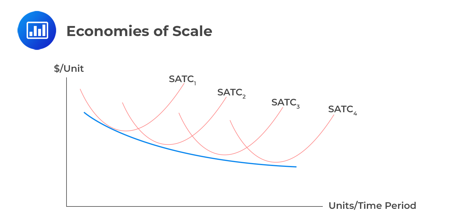
The following factors can lead to economies of scale:

• Achieving economies of scale through increasing returns to scale means the production process yields output increases proportionately larger than the increase in inputs.
• Implementing a division of labor and management to allow workers to specialize in specific tasks, leading to improved job proficiency.
• Enhancing productivity by investing in more expensive and efficient equipment.
• Effectively reducing waste and lowering costs by capitalizing on marketable by-products, reducing energy consumption, and implementing enhanced quality control measures.
• Utilizing market information and knowledge to make more effective managerial decisions.
• Capitalizing on discounted prices when purchasing resources in larger quantities.

Conversely, diseconomies of scale occur when the cost per unit rises as the firm further increases its production. This implies that LRAC has a positive slope. Consider the following graph with SATC for each level of capital input (levels 1,2,3 and 4) in the case of diseconomies of scale:

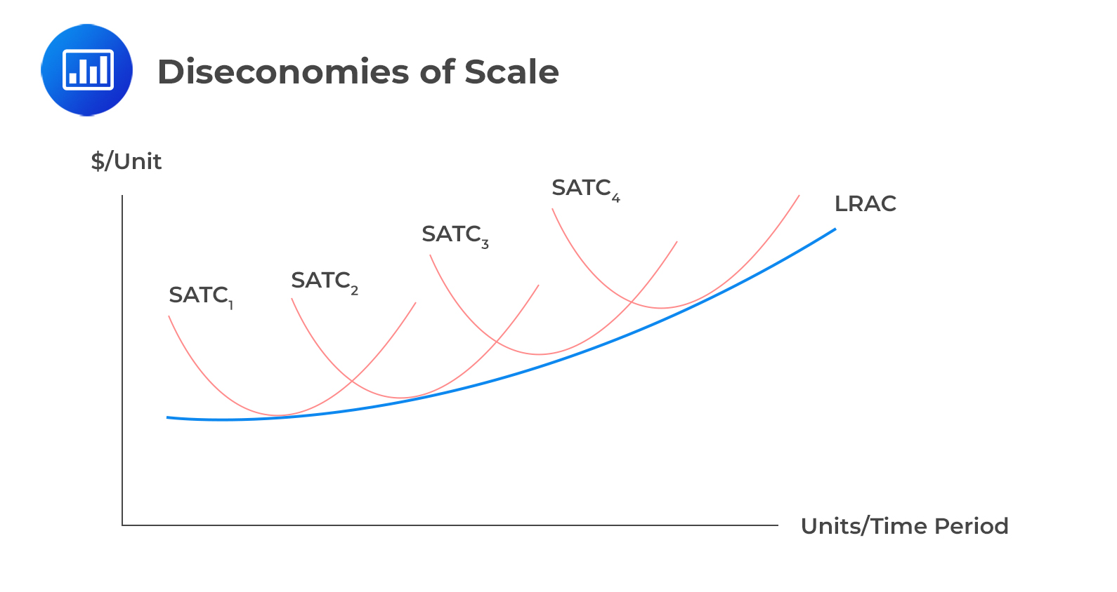
The following factors can result in diseconomies of scale:

• Experiencing diseconomies of scale due to decreasing returns, where the production process results in output increases that are proportionately smaller than the increase in inputs.
• Struggling with proper management due to excessive size.
• Encountering inefficiencies caused by overlapping and duplicating business functions and product lines.
• Facing higher resource prices due to supply constraints when purchasing inputs in large quantities.

Economies of scale and diseconomies of scale can coexist; their effect on the long-run average total cost (LRAC) depends on which one has a stronger influence.

If the economies of scale are more influential, the LRAC will decline as output increases. Conversely, if diseconomies of scale are more prevalent, the opposite happens. It’s possible for the LRAC to first decrease (due to economies of scale) over a certain output range, then stabilize over another range, and subsequently increase in a range where diseconomies of scale take effect.

Theoretically speaking, perfect competition compels a firm to function at the lowest point of the long-run average total cost (LRAC) curve. This is because, over the long term, the market price will settle at this point. If a firm doesn’t operate at this optimal cost-efficiency point, its sustainability in the long run could be at risk.

Question #1

A firm that increases the quantity it produces without any change in per-unit cost is experiencing:

1. Economies of scale.
2. Diseconomies of scale.
3. Constant returns to scale.

Solution

The correct answer is C.

An increase in output proportional to an increase in input would be considered a constant return to scale. This is neither an economies nor diseconomies of scale.

Question #2

The short-term shut-down point of production for a firm operating under perfect competition will most likely occur when the price per unit is equal to:

1. Marginal cost per unit.
2. Average total cost per unit.
3. Average variable cost per unit.

Solution

The correct answer is C.

Any firm will shut down its production when the marginal cost is less than the average variable cost. We will see later that for a firm in perfect competition to maximize profit, marginal revenue must be equal to marginal cost.