Index Construction and Index Returns: Price, Equal, Market-Cap, Float, and Fundamental Weighting

Why Index Construction Matters

A security market index is a financial indicator designed to summarize the performance of a selected group of securities. It may represent a broad market, a sector, an asset class, an investment style, or a custom theme. In modern investment management, indexes do more than report market performance. They also serve as benchmarks for active managers and as blueprints for index funds, exchange-traded funds, and other passive strategies.

The construction of an index is never neutral. A market-capitalization-weighted index gives the greatest influence to the largest companies. An equal-weighted index gives every constituent the same starting influence. A price-weighted index is most affected by securities with high nominal prices. A fundamental-factor-weighted index is shaped by accounting or economic variables such as earnings, revenues, dividends, or book value.

The learning objective therefore requires more than calculation. Candidates must be able to explain how the index design choice affects the index value, the index return, the securities that drive performance, and the portfolio management implications.

The Index Construction Process

Figure 1: Index Construction, Calculation, and Management Process

Figure 1 shows that index construction starts with a purpose. The index provider must first define what the index is intended to represent. After that, the provider selects constituents, assigns weights, calculates the index value, and maintains the index through rebalancing, reconstitution, and adjustments for corporate actions. Each step affects the final index return. A clean-energy infrastructure index, for example, may look very different from a broad-market index even if both contain some of the same securities.

A well-constructed index should answer five practical questions:

• What market, sector, theme, or strategy is being represented?
• Which securities qualify for inclusion?
• How much weight should each security receive?
• How will the index level and returns be calculated?
• How will the index be maintained as prices, shares, fundamentals, and constituents change?

Price Return and Total Return Indexes

A price return index measures changes in constituent prices only. It ignores dividends, coupons, and other capital distributions unless those distributions are reflected in prices.

The price return on an index is:

$$r_{\text{price,index}} = \frac{I_{t+1}^P}{I_t^P} – 1$$

Where:

• \(r_{\text{price,index}}=\) index price return
• \(I_t^P=\) price return index level at time \(t\)
• \(I_{t+1}^P=\) price return index level at time \(t + 1\)

A total return index measures the effect of price changes plus the reinvestment of capital distributions. It is the more complete measure when constituents pay dividends, coupons, or other distributions.

For a single constituent, total return can be expressed as:

$$r_{\text{total}} = \frac{P_{t+1} + D_{t+1}}{P_t} – 1$$

Where:

• \(r_{\text{total}}=\) total return on the constituent
• \(P_t=\) price at time \(t\)
• \(P_{t+1}=\) price at time \(t + 1\)
• \(D_{t+1}=\) capital distribution received over the period

The distinction becomes important over long horizons. Price return indexes show only capital appreciation. Total return indexes show the effect of reinvesting distributions and therefore usually grow faster over time when constituents make positive distributions.

General Index Value

In its most general form, an index can be viewed as a weighted portfolio of constituent prices:

$$I_t = \sum_{i=1}^{N} w_{i,t} P_{i,t}$$

Where:

• \(I_t=\) index value at time \(t\)
• \(N=\) number of constituents in the index
• \(w_{i,t}=\) weight assigned to constituent \(i\) at time \(t\)
• \(P_{i,t}=\) price of constituent \(i\) at time \(t\)

This general formula is useful conceptually, but actual index calculations often use a divisor. The divisor scales the aggregate reference value to a convenient index level, such as 100 or 1,000, and is adjusted when corporate actions or constituent changes would otherwise distort the index.

A divisor-based index value can be expressed as:

$$I_t = \frac{\text{Aggregate reference value}_t}{D_t}$$

Where:

• \(I_t=\) index value at time \(t\)
• \(\text{Aggregate reference value}_t=\) total value determined by the index methodology
• \(D_t=\) index divisor at time \(t\)

The aggregate reference value depends on the weighting method. For a market-capitalization-weighted index, it is total market capitalization. For a price-weighted index, it is the sum of constituent prices. For an equal-weighted index, it is the value of the constructed equal-weighted portfolio.

Major Index-Weighting Methods

Figure 2: How Weighting Methods Shape Index Performance

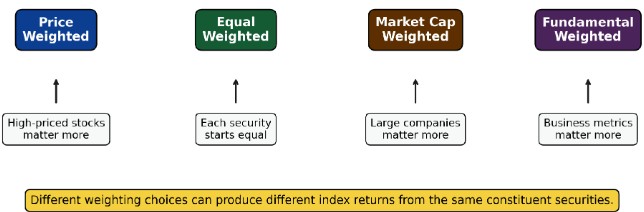
Figure 2 summarizes the main idea. The same securities can produce different index returns depending on how the securities are weighted. A high-return small company may materially affect an equal-weighted index but have little effect on a market-capitalization-weighted index. A high-priced stock can dominate a price-weighted index even if it is not the largest company by market value. A fundamental-weighted index shifts attention from market price to economic scale.

$$ \textbf{Table 1: Major Index-Weighting Methods} \\
\begin{array}{l|c|c|c}
\textbf{Weighting Method} & {\textbf{What Determines} \\ \textbf{the Weight?}} & \textbf{Main Strength} & \textbf{Main Limitation} \\ \hline
\text{Price weighted} & \text{Security price} & {\text{Simple to compute and} \\ \text{understand}} & {\text{High-priced securities} \\ \text{dominate, regardless of} \\ \text{economic size}} \\ \hline
\text{Equal weighted} & {\text{Same starting weight for} \\ \text{every constituent}} & {\text{Reduces concentration in} \\ \text{the largest companies}} & {\text{Requires regular} \\ \text{rebalancing and can} \\ \text{increase turnover}} \\ \hline
{\text{Market capitalization} \\ \text{weighted}} & {\text{Market value of each} \\ \text{company}} & {\text{Reflects the investable} \\ \text{market and needs less} \\ \text{rebalancing}} & {\text{Can become} \\ \text{concentrated in large or} \\ \text{recently appreciated} \\ \text{securities}} \\ \hline
{\text{Float-adjusted market} \\ \text{capitalization weighted}} & {\text{Market value available to} \\ \text{public investors}} & {\text{Better reflects investable} \\ \text{securities}} & {\text{Requires float data and} \\ \text{adjustments}} \\ \hline
{\text{Fundamental-factor} \\ \text{weighted}} & {\text{Accounting or economic} \\ \text{factor such as revenue,} \\ \text{earnings, dividends, or} \\ \text{assets}} & {\text{Links weights to} \\ \text{economic size rather than} \\ \text{market sentiment}} & {\text{Requires fundamental} \\ \text{data and can create} \\ \text{sector or style tilts}} \\
\end{array}
$$

Table 1 is a compact exam checklist. Most questions are not testing whether one method is universally superior. They are testing whether the candidate understands the trade-off created by the weighting choice.

Market-Capitalization-Weighted Indexes

A market-capitalization-weighted index assigns each constituent a weight based on its total market value. A company with a larger market capitalization receives a larger weight and therefore has more influence on the index.

The market-capitalization weight of security \(i\) is:

$$w_i^M = \frac{Q_i P_i}{\sum_{j=1}^{N} Q_j P_j}$$

Where:

• \(w_i^M=\) market-capitalization weight of security \(i\)
• \(Q_i=\) number of shares or units outstanding for security \(i\)
• \(P_i=\) price per share or unit of security \(i\)
• \(\sum_{j=1}^{N} Q_j P_j=\) total market capitalization of all constituents

The value of a market-capitalization-weighted index is:

$$I_t^M = \frac{\sum_{i=1}^{N} Q_i P_{i,t}}{D_t}$$

Where:

• \(I_t^M=\) market-capitalization-weighted index value at time \(t\)
• \(Q_i=\) number of shares or units outstanding for security \(i\)
• \(P_{i,t}=\) price of security \(i\) at time \(t\)
• \(D_t=\) divisor

A key benefit of market-capitalization weighting is that it requires less routine rebalancing than equal weighting, as weights naturally adjust with market values. The main weakness is concentration. If a handful of large companies rise sharply, the index can become heavily exposed to those companies.

Float-Adjusted Market-Capitalization Weighting

Many indexes use only the securities available to the investing public. Shares held by governments, founders, parent companies, or other strategic holders may not be part of the practical investable market. The float adjustment accounts for this issue.

The float-adjusted market-capitalization weight is:

$$w_i^{M,\text{Float}} = \frac{f_i Q_i P_i}{\sum_{j=1}^{N} f_j Q_j P_j}$$

Where:

• \(w_i^{M,\text{Float}}=\) float-adjusted market-capitalization weight of security \(i\)
• \(f_i=\) float factor, or the proportion of shares available to public investors
• \(Q_i=\) number of shares outstanding
• \(P_i=\) price per share
• \(\sum_{j=1}^{N} f_j Q_j P_j=\) total float-adjusted market capitalization of the index

The float-adjusted index value is:

$$I_t^{M,\text{Float}} = \frac{\sum_{i=1}^{N} f_i Q_i P_{i,t}}{D_t}$$

Where:

• \(I_t^{M,\text{Float}}=\) float-adjusted market-capitalization-weighted index value
• \(D_t=\) divisor

The float adjustment is important because it better captures what investors can actually buy. A company may have a large total market capitalization, but if a controlling owner locks up most shares, the freely investable portion may be much smaller.

Example 1: Calculating Market-Capitalization and Float-Adjusted Weights

Suppose we wish to construct an index of four publicly listed payment technology companies. The objective is to compare ordinary market-capitalization weights with float-adjusted weights. Consider the following data:

$$
\begin{array}{l|c|c|c}
\textbf{Security} & \textbf{Shares Outstanding} & \textbf{Price} & \textbf{Float} \\ \hline
\text{A} & {2,000} & {80} & {90\%} \\ \hline
\text{B} & {5,000} & {24} & {100\%} \\ \hline
\text{C} & {4,000} & {35} & {50\%} \\ \hline
\text{D} & {1,000} & {120} & {70\%} \\
\end{array}
$$

Solution

Recall the market-capitalization weight formula is given by:

$$w_i^M = \frac{Q_i P_i}{\sum_{j=1}^{N} Q_j P_j}$$

Where:

• \(Q_i=\) number of shares outstanding for security \(i\)
• \(P_i=\) price of security \(i\)
• \(Q_i P_i=\) market capitalization of security \(i\)
• \(\sum_{j=1}^{N} Q_j P_j=\) total market capitalization across all four securities

The market capitalizations are:

$$
\begin{array}{l|c}
\textbf{Security} & \textbf{Market Capitalization} \\ \hline
\text{A} & {160,000} \\ \hline
\text{B} & {120,000} \\ \hline
\text{C} & {140,000} \\ \hline
\text{D} & {120,000} \\ \hline
\text{Total} & {540,000} \\
\end{array}
$$

The market-capitalization weights are:

$$
\begin{align}
w_A^M &= \frac{160,000}{540,000} = 29.63\% \\
w_B^M &= \frac{120,000}{540,000} = 22.22\% \\
w_C^M &= \frac{140,000}{540,000} = 25.93\% \\
w_D^M &= \frac{120,000}{540,000} = 22.22\%
\end{align}
$$

Now use the float-adjusted formula:

$$w_i^{M,\text{Float}} = \frac{f_i Q_i P_i}{\sum_{j=1}^{N} f_j Q_j P_j}$$

Where:

• \(f_i=\) proportion of shares in the public float
• \(f_i Q_i P_i=\) float-adjusted market capitalization

The float-adjusted market capitalizations are:

$$
\begin{array}{l|c|c}
\textbf{Security} & {\textbf{Float-Adjusted} \\ \textbf{Market Capitalization}} & {\textbf{Float-Adjusted} \\ \textbf{Weight}} \\ \hline
\text{A} & {144,000} & {34.45\%} \\ \hline
\text{B} & {120,000} & {28.71\%} \\ \hline
\text{C} & {70,000} & {16.75\%} \\ \hline
\text{D} & {84,000} & {20.10\%} \\ \hline
\text{Total} & {418,000} & {100.00\%} \\
\end{array}
$$

Security C has a sizable total market capitalization, but only half of its shares are in the public float. Its weight therefore falls from 25.93% under ordinary market-capitalization weighting to 16.75% under float-adjusted weighting. That change is economically meaningful: the index gives less influence to a security that is less available to public investors.

Example 2: Calculating a Float-Adjusted Index Price Return and Total Return

Suppose we want to calculate the price return and total return of the float-adjusted index from Example 1. The initial divisor is set so that the index begins at 100:

$$D_0 = \frac{418,000}{100} = 4,180$$

At the end of the period, prices and distributions are as follows:

$$
\begin{array}{l|c|c|c}
\textbf{Security} & \textbf{Initial Price} & \textbf{Ending Price} & \textbf{Distribution} \\ \hline
\text{A} & {80} & {88} & {1.20} \\ \hline
\text{B} & {24} & {22} & {0.80} \\ \hline
\text{C} & {35} & {42} & {0.50} \\ \hline
\text{D} & {120} & {114} & {2.00} \\
\end{array}
$$

Solution

Recall that:

$$I_t^{M,\text{Float}} = \frac{\sum_{i=1}^{N} f_i Q_i P_{i,t}}{D_t}$$

Where:

• \(I_t^{M,\text{Float}}=\) float-adjusted index value
• \(f_i=\) float factor for security \(i\)
• \(Q_i=\) number of shares outstanding
• \(P_{i,t}=\) price of security \(i\) at time \(t\)
• \(D_t = 4,180=\) divisor

Using ending prices only, the aggregate float-adjusted value is:

$$0.90(2,000)(88) + 1.00(5,000)(22) + 0.50(4,000)(42) + 0.70(1,000)(114) = 432,200$$

The ending price index level is:

$$I_1^P = \frac{432,200}{4,180} = 103.40$$

The price return is:

$$r_{\text{price,index}} = \frac{103.40}{100} – 1 = 3.40\%$$

For the total return version, include distributions:

$$I_1^{TR} = \frac{\sum_{i=1}^{N} f_i Q_i (P_{i,1} + D_{i,1})}{D_0}$$

Where:

• \(I_1^{TR}=\) total return index level at the end of the period
• \(D_{i,1}=\) distribution paid by security \(i\) during the period

The total-return aggregate value is:

$$ \begin{align*} & 0.90(2,000)(89.20) + 1.00(5,000)(22.80) + 0.50(4,000)(42.50) + 0.70(1,000)(116.00) \\ & = 440,760 \end{align*} $$

The total return index level is:

$$I_1^{TR} = \frac{440,760}{4,180} = 105.45$$

The total return is:

$$r_{\text{total,index}} = \frac{105.45}{100} – 1 = 5.45\%$$

The total return exceeds the price return because the total return index assumes that distributions are reinvested into the index.

Equal-Weighted Indexes

An equal-weighted index assigns the same starting weight to each constituent. If the index has \(N\) securities, each constituent initially receives a weight of \(1/N\).

The equal weight of each constituent is:

$$w_i^E = \frac{1}{N}$$

Where:

• \(w_i^E=\) equal weight assigned to security \(i\)
• \(N=\) number of constituents

When all constituents are equally weighted at the start of the period, the one-period price return of the index can be calculated as the average of the constituent price returns:

$$r_{\text{index}}^E = \frac{1}{N} \sum_{i=1}^{N} r_i$$

Where:

• \(r_{\text{index}}^E=\) equal-weighted index return
• \(r_i=\) return on security \(i\)
• \(N=\) number of constituents

Equal weighting reduces concentration in the largest companies, but it creates a need for regular rebalancing. If one stock rises sharply, it becomes more than an equal-weight position; if another falls sharply, it becomes less than an equal-weight position. Restoring equal weights requires selling some winners and buying some laggards.

Example 3: Comparing Equal-Weighted and Price-Weighted Returns

Assume we would like to calculate the price return on an equal-weighted index using the ending prices from Example 2. The four constituent price returns are:

$$
\begin{array}{l|c|c|c} \textbf{Security} & \textbf{Initial Price} & \textbf{Ending Price} & \textbf{Price Return} \\ \hline
\text{A} & {80} & {88} & {10.00\%} \\ \hline
\text{B} & {24} & {22} & {-8.33\%} \\ \hline
\text{C} & {35} & {42} & {20.00\%} \\ \hline
\text{D} & {120} & {114} & {-5.00\%} \\
\end{array}
$$

Solution

The equal-weighted return is given by:

$$r_{\text{index}}^E = \frac{1}{N} \sum_{i=1}^{N} r_i$$

Where:

• \(N = 4\), the number of securities in the index
• \(r_A = 10.00\%\), \(r_B = -8.33\%\), \(r_C = 20.00\%\), and \(r_D = -5.00\%\)
• \(r_{\text{index}}^E\) is the equal-weighted index price return

Substituting the returns:

$$r_{\text{index}}^E = \frac{10.00\% – 8.33\% + 20.00\% – 5.00\%}{4} = 4.17\%$$

Now compare this with a price-weighted index using the same four securities.

A price-weighted index is calculated as:

$$I_t^P = \frac{\sum_{i=1}^{N} P_{i,t}}{D_t}$$

Where:

• \(I_t^P=\) price-weighted index level
• \(P_{i,t}=\) is the price of security \(i\) at time \(t\)
• \(D_t=\) divisor

At the start of the period, the sum of prices is:

$$80 + 24 + 35 + 120 = 259$$

If the divisor is set to 2.59, the initial index level is 100. At the end of the period, the sum of prices is:

$$88 + 22 + 42 + 114 = 266$$

The ending price-weighted index level is:

$$I_1^P = \frac{266}{2.59} = 102.70$$

The price-weighted index return is:

$$r_{\text{price,index}} = \frac{102.70}{100} – 1 = 2.70\%$$

The equal-weighted index return is higher than the price-weighted index return because Security C had a strong return and receives a full 25% weight in the equal-weighted index. In the price-weighted index, Security C has less influence than Security D because its nominal price is lower.

Fundamental-Factor-Weighted Indexes

A fundamental-factor-weighted index assigns weights based on economic or accounting measures rather than on market prices alone. Common examples include revenues, earnings, book value, cash flow, dividends, or a composite of several such measures.

The fundamental-factor weight is:

$$w_i^F = \frac{F_i}{\sum_{j=1}^{N} F_j}$$

Where:

• \(w_i^F=\) fundamental-factor weight of security \(i\)
• \(F_i=\) selected fundamental measure for security \(i\)
• \(\sum_{j=1}^{N} F_j=\) total fundamental reference value across all constituents

Fundamental weighting can be useful when investors want an index that reflects economic footprint rather than current market sentiment. A revenue-weighted index, for example, may give greater weight to companies with large sales even if their market prices have recently lagged. This design can create style, sector, and valuation tilts, so it should be interpreted carefully.

Example 4: Calculating Fundamental-Factor Weights

Suppose we want to construct a revenue-weighted index for four cloud-computing firms. The latest annual revenues are:

$$
\begin{array}{l|c}
\textbf{Security} & \textbf{Revenue} \\ \hline
\text{A} & {9.0} \\ \hline
\text{B} & {4.0} \\ \hline
\text{C} & {5.0} \\ \hline
\text{D} & {2.0} \\
\end{array}
$$

Recall that:

$$w_i^F = \frac{F_i}{\sum_{j=1}^{N} F_j}$$

Where:

• \(F_i=\) revenue for company \(i\)
• \(\sum_{j=1}^{N} F_j = 20.0\), total revenue across the four companies
• \(w_i^F=\) revenue-based fundamental weight

The weights are:

$$
\begin{align}
w_A^F &= \frac{9.0}{20.0} = 45.0\% \\
w_B^F &= \frac{4.0}{20.0} = 20.0\% \\
w_C^F &= \frac{5.0}{20.0} = 25.0\% \\
w_D^F &= \frac{2.0}{20.0} = 10.0\%
\end{align}
$$

Company A receives the largest weight because it has the largest revenue base. If the index were market-cap weighted, the largest weight might go to a different company if investors assigned that company a higher valuation. That is the core conceptual difference: fundamental weighting emphasizes business scale, while market-capitalization weighting emphasizes market value.

Price-Weighted Indexes and Divisor Adjustments

A price-weighted index gives more influence to securities with higher nominal prices:

$$w_i^P = \frac{P_i}{\sum_{j=1}^{N} P_j}$$

Where:

• \(w_i^P=\) price weight of security \(i\)
• \(P_i=\) price of security \(i\)
• \(\sum_{j=1}^{N} P_j=\) sum of prices across all constituents

A practical issue arises when a company undergoes a stock split. A two-for-one stock split halves the price per share but does not, by itself, destroy shareholder wealth. If the divisor is not adjusted, the index would mechanically decline even though the company’s economic value has not changed.

The divisor can be adjusted as follows:

$$D_{\text{new}} = \frac{\sum_{i=1}^{N} P_{i,\text{post action}}}{I_{\text{pre action}}}$$

Where:

• \(D_{\text{new}}=\) adjusted divisor
• \(\sum_{i=1}^{N} P_{i,\text{post action}}=\) sum of constituent prices immediately after the corporate action
• \(I_{\text{pre action}}=\) index level immediately before the corporate action

Example 5: Adjusting the Divisor After a Stock Split

Suppose we want to maintain the continuity of a price-weighted index after a two-for-one stock split. Before the split, the index contains four securities priced at 80, 24, 35, and 120. The divisor is 2.59, so the index level is:

$$I_{\text{pre action}} = \frac{80 + 24 + 35 + 120}{2.59} = 100$$

Security D then has a two-for-one split, reducing its price from 120 to 60. The economic value of investors’ holdings has not changed, so the index should remain at 100 immediately after the split.

Start by quoting the divisor adjustment formula:

$$D_{\text{new}} = \frac{\sum_{i=1}^{N} P_{i,\text{post action}}}{I_{\text{pre action}}}$$

Where:

• \(\sum_{i=1}^{N} P_{i,\text{post action}} = 80 + 24 + 35 + 60 = 199\)
• \(I_{\text{pre action}} = 100\)
• \(D_{\text{new}}=\) new divisor

Substitute the values:

$$D_{\text{new}} = \frac{199}{100} = 1.99$$

The divisor must be changed from 2.59 to 1.99. Without the divisor adjustment, the price-weighted index would appear to fall, even though the split by itself did not create an economic loss.

Index Management: Rebalancing and Reconstitution

Rebalancing means adjusting constituent weights back toward the index’s target weighting method. Equal-weighted indexes and fundamental-factor-weighted indexes typically require periodic rebalancing because market price changes cause weights to drift away from target weights.

Reconstitution means changing the index membership. A company may be added because it now meets the eligibility rules, or removed because it no longer qualifies. Reconstitution is necessary to keep the index aligned with its stated objective.

A key distinction is that rebalancing changes weights, while reconstitution changes constituents.

$$ \textbf{Table 2: Rebalancing and Reconstitution} \\
\begin{array}{l|c|c}
\textbf{Process} & \textbf{What Changes?} & \textbf{Why It Matters} \\ \hline
\text{Rebalancing} & \text{Constituent weights} & {\text{Restores intended exposure and} \\ \text{controls weight drift}} \\ \hline
\text{Reconstitution} & \text{Constituent membership} & {\text{Keeps the index aligned with the} \\ \text{target market, sector, or strategy}} \\ \hline
\text{Divisor adjustment} & \text{Divisor used in index calculation} & {\text{Preserves index continuity around} \\ \text{non-return events such as splits or} \\ \text{constituent changes}} \\
\end{array}
$$

Table 2 connects index management to the interpretation of returns. A change in index level should reflect investment performance, not a purely mechanical event such as a split or a constituent replacement. Divisor adjustments help preserve that continuity.

Interpretation and Evaluation

Several practical principles follow:

• Price return indexes exclude distributions; total return indexes include reinvested distributions.
• Market-capitalization weighting gives more influence to companies with larger market value.
• Float adjustment reduces the weight of securities that are not freely available to public investors.
• Equal weighting reduces large-company concentration but requires regular rebalancing.
• Price weighting can be distorted by high nominal prices and stock splits.
• Fundamental weighting links weights to economic or accounting measures.
• Rebalancing changes weights; reconstitution changes membership.
• Divisor adjustments preserve index continuity when non-return events occur.

Question

A market-capitalization-weighted index contains three stocks:

$$
\begin{array}{l|c|c|c|c}
\textbf{Stock} & \textbf{Shares Outstanding} & \textbf{Initial Price} & \textbf{Ending Price} & \textbf{Dividend} \\ \hline
\text{A} & {1,000} & {50} & {55} & {1.00} \\ \hline
\text{B} & {2,000} & {20} & {18} & {0.50} \\ \hline
\text{C} & {500} & {80} & {92} & {2.00} \\
\end{array}
$$

The divisor is set so that the initial index value is 100. The index’s price return and total return are closest to:

1. 5.38% and 5.38%
2. 5.38% and 7.69%
3. 7.69% and 5.38%

Answer Explanation

The correct answer is B.

Start by quoting the market-capitalization-weighted index formula:

$$I_t^M = \frac{\sum_{i=1}^{N} Q_i P_{i,t}}{D_t}$$

Where:

• \(I_t^M\) is the market-capitalization-weighted index value
• \(Q_i\) is the shares outstanding for stock \(i\)
• \(P_{i,t}\) is the price of stock \(i\) at time \(t\)
• \(D_t\) is the divisor
• \(N = 3\), the number of stocks

The initial aggregate market capitalization is:

$$(1,000)(50) + (2,000)(20) + (500)(80) = 130,000$$

Because the initial index value is 100, the divisor is:

$$D_0 = \frac{130,000}{100} = 1,300$$

Using ending prices only, the new aggregate market capitalization is:

$$(1,000)(55) + (2,000)(18) + (500)(92) = 137,000$$

The ending price index level is:

$$I_1^P = \frac{137,000}{1,300} = 105.38$$

The price return is:

$$r_{\text{price,index}} = \frac{105.38}{100} – 1 = 5.38\%$$

For the total return, include the dividends:

$$I_1^{TR} = \frac{\sum_{i=1}^{N} Q_i (P_{i,1} + D_{i,1})}{D_0}$$

Where:

• \(I_1^{TR}=\) total return index level
• \(D_{i,1}=\) dividend paid by stock \(i\) during the period

The dividend-adjusted aggregate value is:

$$(1,000)(56) + (2,000)(18.50) + (500)(94) = 140,000$$

The total return index level is:

$$I_1^{TR} = \frac{140,000}{1,300} = 107.69$$

The total return is:

$$r_{\text{total,index}} = \frac{107.69}{100} – 1 = 7.69\%$$

The price return is 5.38%, and the total return is 7.69%.

A is incorrect because it ignores dividends and therefore reports the price return as both the price return and the total return.

C is incorrect because it reverses the price return and the total return. The total return should exceed the price return when dividends are positive and reinvesting.