




Uncorrelated Portfolio Holdings
The portfolio standard deviation, or risk, is not simply the addition of the... Read More

Investment performance is not measured in a vacuum. A portfolio may receive additional contributions, make distributions, experience withdrawals, and change in value between those cash-flow events. When those flows are large, the investor’s final wealth may depend not only on the portfolio’s investment returns but also on when capital was invested or withdrawn.
This is why two investors can hold exposure to the same investment strategy and yet experience different returns. One investor may contribute capital just before a strong period, while another may contribute just before a weak period. The underlying portfolio may have the same subperiod returns in both cases, but the investor experience can differ substantially.
The key distinction in this learning outcome is therefore straightforward:
This distinction is especially important in performance evaluation. Public-market managers typically do not control client contributions and withdrawals, so their skill is usually evaluated using time-weighted returns. Investors, however, often care more about the return earned on their actual money, which is captured by money-weighted returns.
An external cash flow is a contribution to or withdrawal from the portfolio that is controlled by the investor rather than generated by the portfolio’s investment activity. Dividends, interest income, and realized gains can be reinvested inside the portfolio and may be part of investment performance. By contrast, a new client contribution or a client withdrawal changes the amount of money invested and can distort return measurement if not handled carefully.
Figure 1: Cash Flow Timing and Return Measurement
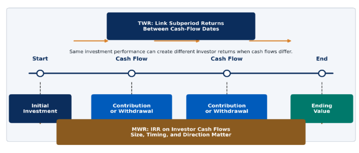
Figure 1 shows why the timing of cash flows matters. Time-weighted return divides the full evaluation period into subperiods around cash-flow events and then links the subperiod returns. This structure reduces the effect of external cash flows on the performance measure. Money-weighted return instead treats the investment as a series of dated cash inflows and outflows and calculates the internal rate of return on those flows.
The time-weighted rate of return measures the compound rate of growth of an investment over a specified period after removing the distorting effect of external cash flows. It does this by splitting the full evaluation period into subperiods at each external cash-flow date, calculating each subperiod return, and then geometrically linking those returns.
The time-weighted rate of return over the full measurement period is:
$$r_{TW} = \prod_{t=1}^{T} (1 + r_t) – 1$$
Where:
The result is a compound return for the full period. When the period covers one year, the result is the annual time-weighted return. When the subperiods cover several years, the annualized time-weighted return is calculated as the geometric mean of the linked annual returns:
$$r_{TW,\text{annualized}} = \left[ \prod_{t=1}^{T} (1 + r_t) \right]^{1/T} – 1$$
Where:
The time-weighted measure is especially useful when evaluating an investment manager who does not control the timing or size of investor contributions and withdrawals. It asks, in effect, “How did the investment strategy perform per unit of capital invested throughout the period?”
Example 1: Calculating Time-Weighted Return
Suppose we wish to calculate the time-weighted return for a public equity portfolio over a year. The portfolio is valued immediately before each external cash flow, and the three subperiod returns are as follows:
$$\begin{array}{l|c}
\textbf{Subperiod} & \textbf{Portfolio Return} \\ \hline
\text{January–April} & 7.0\% \\ \hline
\text{May–August} & -3.0\% \\ \hline
\text{September–December} & 6.0\% \\
\end{array}$$
The objective is to measure the portfolio’s underlying performance, not the effect of investor contributions or withdrawals.
Solution
Recall that:
$$r_{TW} = \prod_{t=1}^{T} (1 + r_t) – 1$$
Where:
Substitute the subperiod returns:
$$\begin{align}
r_{TW} &= (1.07)(0.97)(1.06) – 1 \\
r_{TW} &= 1.1007 – 1 = 10.07\%
\end{align}$$
The time-weighted return is 10.07%. This return reflects the compounded investment performance across the three subperiods. It is not affected by whether investors contributed a large or small amount during one of the subperiods.
The money-weighted rate of return, also called the dollar-weighted rate of return, is the internal rate of return on the investment’s actual cash flows. It is the discount rate that sets the present value of all cash inflows and outflows equal to zero:
$$0 = \sum_{t=0}^{T} \frac{CF_t}{(1 + r_{MW})^t}$$
Where:
The money-weighted rate is usually calculated using a financial calculator, the spreadsheet IRR function, or a numerical method. It generally does not have a simple direct algebraic solution when there are multiple interim cash flows.
The money-weighted return answers a different question from the time-weighted return. It asks, “What return did the investor actually earn on the money invested, considering when each cash flow occurred?”
$$ \textbf{Table 1: Time-Weighted and Money-Weighted Return Compared} \\
\begin{array}{l|c|c}
\textbf{Feature} & \textbf{Time-Weighted Return} & \textbf{Money-Weighted Return} \\ \hline
\text{Main purpose} & {\text{Evaluates investment} \\ \text{strategy performance}} & {\text{Evaluates the return earned on} \\ \text{actual investor capital}} \\ \hline
{\text{Treatment of external} \\ \text{cash flows}} & {\text{Removes the effect of timing and} \\ \text{size by calculating subperiod} \\ \text{returns}} & {\text{Directly incorporates timing and} \\ \text{size of cash flows}} \\ \\ \hline
\text{Calculation method} & {\text{Geometrically links subperiod} \\ \text{returns}} & {\text{Solves for the internal rate of} \\ \text{return}} \\ \hline
\text{Most useful for:} & {\text{Public-market manager} \\ \text{performance evaluation}} & {\text{Investor experience and} \\ \text{private-market performance } \\ \text{evaluation when the manager} \\ \text{controls cash flows}} \\ \hline
{\text{Can differ} \\ \text{materially when:}} & {\text{External cash flows are large or} \\ \text{occur before strong or weak} \\ \text{performance}} & {\text{External cash flows are large or} \\ \text{occur before strong or weak} \\ \text{performance}} \\
\end{array}$$
Table 1 is central to the learning outcome. Neither measure is automatically “better” in all situations. The correct measure depends on the question being asked. If the goal is to isolate the manager’s investment decisions from client cash flows, time-weighted return is usually appropriate. If the goal is to measure the investor’s actual return on invested capital, money-weighted return is usually more relevant.
Example 2: Calculating Money-Weighted Return
Suppose an investor in a private infrastructure fund contributes USD 80 million at inception and an additional USD 40 million after four months. The investor receives no interim distributions over the next four months and receives only USD 128.84 million at the end of the year.
From the investor’s perspective, the cash flows are:
$$
\begin{array}{l|c}
\textbf{Time} & \textbf{Cash Flow} \\ \hline
0 & -80.00 \\ \hline
1 & -40.00 \\ \hline
2 & 0.00 \\ \hline
3 & 128.84 \\
\end{array}
$$
Calculate the money‑weighted rate of return for this investment.
Solution
The objective is to calculate the internal rate of return over each four-month interval and then annualize it.
We know that:
$$0 = \sum_{t=0}^{T} \frac{CF_t}{(1 + r_{MW})^t}$$
Where:
Substituting the cash flows:
$$0 = -80 + \frac{-40}{(1 + r_{MW})} + \frac{0}{(1 + r_{MW})^2} + \frac{128.84}{(1 + r_{MW})^3}$$
Solving for the internal rate of return (using a financial calculator) gives:
$$r_{MW} = 2.70\%$$
Because the cash-flow intervals are four months long, there are three such intervals in one year. The annualized money-weighted return is:
$$r_{MW,\text{annualized}} = (1.0270)^3 – 1 = 8.32\%$$
The annualized money-weighted return is 8.32%. The result reflects the investor’s actual cash-flow experience, including the large additional contribution after the first four months.
Time-weighted and money-weighted returns can be equal, but they often differ when cash flows are material. The difference is driven by when large amounts of capital are exposed to strong or weak investment performance.
Suppose the same portfolio in Example 2 generated subperiod returns of 13.0%, -5.0%, and 4.0%. The time-weighted return would be:
$$r_{TW} = (1.13)(0.95)(1.04) – 1 = 11.64\%$$
The money-weighted return from Example 2 was 8.32% on an annualized basis. The time-weighted return is higher because the portfolio performed best before the investor made the large second contribution. A smaller amount of capital participated in the strongest subperiod, while a larger amount participated in the later, weaker subperiods.
This comparison is not a contradiction. The two measures are answering different questions. The time-weighted return describes the portfolio’s underlying investment performance. The money-weighted return describes the return earned on the investor’s actual invested capital.
$$ \textbf{Table 2: When to Prefer Each Return Measure} \\
\begin{array}{l|c|c}
\textbf{Situation} & \textbf{More Relevant Measure} & \textbf{Reason} \\ \hline
{\text{Public equity manager receives} \\ \text{unpredictable client contributions} \\ \text{and withdrawals}} & \text{Time-weighted return} & {\text{The manager usually does not} \\ \text{control external client cash flows}} \\ \hline
{\text{Investor wants to know the return} \\ \text{earned on personal contributions} \\ \text{and withdrawals}} & \text{Money-weighted return} & {\text{The measure incorporates the} \\ \text{size and timing of the investor’s} \\ \text{cash flows}} \\ \hline
{\text{Private equity manager controls} \\ \text{capital calls and distributions}} & \text{Money-weighted return} & {\text{Timing and sizing of cash flows} \\ \text{are part of the manager’s} \\ \text{investment process}} \\ \hline
{\text{Daily-valued mutual fund reports} \\ \text{standardized performance}} & \text{Time-weighted return} & {\text{Daily subperiod returns can be} \\ \text{linked while external flows are} \\ \text{neutralized}} \\
\end{array}
$$
Table 2 gives the practical interpretation. A public-market portfolio manager should not generally be penalized because a client contributed large capital just before a weak market. At the same time, an investor should care about the actual return earned on the capital invested at each date.
Money-weighted return calculations require a clear sign convention. From the investor’s perspective, cash paid into the investment is negative, while cash received from the investment is positive.
$$ \textbf{Table 3: Investor-Perspective Cash-Flow Signs} \\
\begin{array}{l|l|l}
\textbf{Cash Flow} & \textbf{Sign} & \textbf{Explanation} \\ \hline
\text{Initial investment} & \text{Negative} & {\text{The investor gives up cash to} \\ \text{acquire the investment}} \\ \hline
\text{Additional contribution} & \text{Negative} & {\text{The investor adds more} \\ \text{capital}} \\ \hline
\text{Withdrawal} & \text{Positive} & {\text{The investor receives cash} \\ \text{back}} \\ \hline
{\text{Dividend or distribution} \\ \text{paid out to investor}} & \text{Positive} & \text{The investor receives cash} \\ \hline
\text{Ending portfolio} & \text{value Positive} & {\text{The investor could liquidate} \\ \text{the investment for that value}} \\
\end{array}
$$
Table 3 helps prevent one of the most common errors in money-weighted return questions: reversing the signs. A sign reversal may still yield a numerical answer, but it will not represent the investor’s internal rate of return.
In practice, portfolios are often valued daily. Daily valuation improves return measurement because it permits the analyst to calculate daily holding-period returns and link them across the full year:
$$r_{TW} = (1 + r_1)(1 + r_2)\cdots(1 + r_D) – 1$$
Where:
If daily returns are used for a calendar year, \(D\) might be 365. If trading days are used, \(D\) is often approximately 252. The choice of calendar-day or trading-day convention affects the compounded result and should be applied consistently.
For multiple years, annual time-weighted returns are usually geometrically linked:
$$r_{TW,\text{annualized}} = \left[ (1 + r_1)(1 + r_2)\cdots(1 + r_T) \right]^{1/T} – 1$$
Where:
The Global Investment Performance Standards, or GIPS, provide guidance for how investment performance should be presented. The key conceptual point for this learning outcome is the connection between control over cash flows and the appropriate measure of return.
For most public-market strategies, time-weighted returns are preferred because managers do not control when clients top up or withdraw some money. The purpose is to evaluate the manager’s investment decisions without distortion from external flows.
Money-weighted returns may be appropriate when the manager controls the timing and amount of external cash flows, such as in certain private-market structures involving committed capital, capital calls, distributions, illiquid assets, or fixed-life investment vehicles. In such settings, deciding when to call and deploy capital is part of the investment management process.
Several practical points follow:
Question
A portfolio earns subperiod returns of 9.0%, -4.0%, and 5.0% during a year. At the beginning of the year, an investor contributes USD 50 million. After the first subperiod, the investor contributes an additional USD 30 million. No further external cash flows occur until the end of the year.
The portfolio’s time-weighted return for the year is closest to:
- 9.27%
- 9.87%
- 10.00%
Answer Explanation
The correct answer is B.
Recall that the time-weighted return is given by:
$$r_{TW} = \prod_{t=1}^{T} (1 + r_t) – 1$$
Where:
- \(T = 3\), the number of subperiods
- \(r_1 = 9.0\%\), the first subperiod return
- \(r_2 = -4.0\%\), the second subperiod return
- \(r_3 = 5.0\%\), the third subperiod return
- \(r_{TW}\) is the time-weighted return for the year
Substituting the returns:
$$
\begin{align}
r_{TW} &= (1.09)(0.96)(1.05) – 1 \\
r_{TW} &= 1.0987 – 1 = 9.87\%
\end{align}
$$
Master CFA Level I Portfolio Management concepts, including money-weighted return, time-weighted return, portfolio performance measurement, return calculations, and exam-style practice questions with study notes, mock exams, and video lessons.






Get Ahead on Your Study Prep This Cyber Monday! Save 35% on all CFA® and FRM® Unlimited Packages. Use code CYBERMONDAY at checkout. Offer ends Dec 1st.