SOA Exam IFM Prep Notes
Online and Printable Prep Books for Exam IFM
Exam IFM is a three-hour multiple-choice examination designed to build your knowledge of the theoretical elements of corporate finance and financial models. Exam IFM has the most number of topics among all the three preliminary exams – a total of 10. AnalystPrep’s team of academics and practicing actuaries has developped concise prep notes focusing all of the rudimentary aspects of financial markets.
With AnalystPrep’s concise prep notes for Exam IFM, you can simply read on your tablet, computer, or print each concept before jumping into the question bank portion of the platform.
Questions Answered by our Users
Satisfied Customers
preparation platform according to review websites

What are the Ten Topics?
Exam IFM should be taken right after having sat and passed SOA exams P and FM, since financial market concepts have the following foundations:
- Calculus and probability – part of the Exam P syllabus
- Interest theory – found in the Exam FM curriculum
Exam IFM could be further subdivided into three main themes – general finance theories (topics 1 to 3), project analysis and capital structure (topics 4 and 5), and derivatives pricing (topics 6 to 10).
| Topic | Weighting | |
| 1 | Mean-Variance Portfolio Theory | 10-15% |
| 2 | Asset Pricing Models | 5-10% |
| 3 | Market Efficiency and Behavioral Finance | 5-10% |
| 4 | Investment Risk and Project Analysis | 10-15% |
| 5 | Capital Structure | 10% |
| 6 | Introductory Derivatives – Forwards and Futures | 5-10% |
| 7 | General Properties of Options | 10-15% |
| 8 | Binomial Pricing Models | 10% |
| 9 | Black-Scholes Option Pricing Model | 10-15% |
| 10 | Option Greeks and Risk Management | 5-10% |
All of the Content on One Platform

Example Learning Objective from AnalystPrep's SOA Exam IFM Prep Notes
Topic 9: Black Scholes Option Pricing Model
Lognormal Distribution
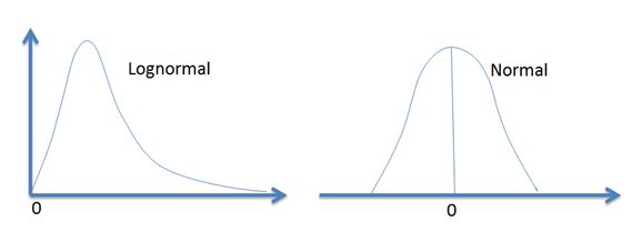
Suppose we have a random variable X. This variable will have a lognormal distribution if its natural log (ln X) is normally distributed. In other words, when the natural logarithm of a random variable is normally distributed, then the variable itself will have a lognormal distribution.
That is,
If X is distributed lognormally, with the parameters \(\mu\) and \(\sigma\) we can write,
\(X \sim \log { N\left( \mu,\sigma^2 \right) } \). The Probability Distribution function is given by:
$$ f(x)=\frac {1}{x \sigma \sqrt{2\pi }} e^{-\frac {1}{2} \left( \frac {logX-\mu}{\sigma} \right)^2 } \text { for } 0 < X < \infty $$
The mean and variance of the lognormal distribution are:
$$ E(X)=e^{\mu+\frac {1}{2} \sigma^2 } $$
And
$$ Var(X)=e^{2\mu+\sigma^2 }{(e^{\sigma^2 }-1)} $$
The two most important characteristics of the lognormal distribution are as follows:
- It has a lower bound of zero, i.e., a lognormal variable cannot take on negative values
- The distribution is skewed to the right, i.e., it has a long right tail.
These characteristics are in direct contrast to those of the normal distribution which is symmetrical (zero skews) and can take on both negative and positive values. As a result, the normal distribution cannot be used to model stock prices because stock prices cannot fall below zero. The lognormal distribution is also used to value options.
 The Lognormal Property of Stock Prices
Black Scholes and Merton employed a model that assumed that percentage changes in the stock price in a short period of time is normally distributed. Now, define the following:
\(\mu\)-expeted return on the stock per year
\(\sigma\)-volatility of the stock price per year
Intuitively, the return in time \(\Delta t\) is \(\mu \Delta t\) and the standard deviation is \(\sigma \sqrt{\Delta t}\). This implies that:
$$ \frac {\Delta S}{S}=\Phi(\mu \Delta t,\sigma^2 \Delta t) $$
where \(\Delta S\) is the change in the stock price at time \(\Delta t\) and \(\Phi(m,v)\) is the normal distribution with the mean m and the variance v.
Without proof, it implies that:
$$ \begin{align*} & lnS_T-lnS_0 \sim \Phi \left[ \left( \mu-\frac {\sigma^2}{2}\right)T,\sigma^2 T \right] \\ \Rightarrow &\frac {lnS_T}{lnS_0} \sim \Phi \left[ \left( \mu-\frac {\sigma^2}{2}\right)T,\sigma^2 T \right] \\ \end{align*} $$
And also
$$ lnS_T \sim \Phi \left[lnS_0+ \left(\mu-\frac {\sigma^2}{2} \right) T,\sigma^2 T \right] $$
The last expression can be written as:
$$ lnS_T \sim N \left[lnS_0+ \left(\mu-\frac {\sigma^2}{2} \right) T,\sigma^2 T \right]…………(1) $$
Where we will concentrate on, where:
\(S_T\)=stock price at time T
\(S_0\)=stock price at time 0
\(\mu\)=expected return on stock per year
\(\sigma\)=annual volatility of the stock price
If we let \(\delta\) be the dividend yield then, (1) becomes:
$$ lnS_T \sim N \left[lnS_0+ \left(\mu- \delta – \frac {\sigma^2}{2} \right) T,\sigma^2 T \right] $$
The subtraction of dividend yield is necessary since higher dividend yield means a lower future stock price.
Note: The above relationship holds because mathematically, if the natural logarithm of a random variable x(lnx) is normally distributed, then xx has a lognormal distribution. It’s also imperative to note that the BSM model assumes stock prices are lognormally distributed, with stock returns being normally distributed. Specifically, continuously compounded annual returns are normally distributed with:
a mean of \(\left[\mu-\frac {\sigma^2}{2} \right]\) and variance of \(\frac {\sigma^2}{T} \)
Example
ABC stock has an initial price of $60, an expected annual return of 10%, and annual volatility of 15%. Calculate the mean and the variance of the distribution of the stock price in six months.
- \(\mu\)=4.139,\(\sigma\)=0.011
- \(\mu\)=3.139,\(\sigma\)=0.211
- \(\mu\)=4.039,\(\sigma\)=0.013
- \(\mu\)=4.139,\(\sigma\)=0.011
- \(\mu\)=2.139,\(\sigma\)=0.211
The correct answer is A.
We know that:
$$ \begin{align*} & lnS_T-lnS_0 \sim \Phi \left[ \left( \mu-\frac {\sigma^2}{2}\right)T,\sigma^2 T \right] \\ & =N \left[ln60+ \left(0.10-\frac {0.15^2}{2} \right)0.5,0.15^2×0.5 \right] \\ & \Rightarrow ` lnS_T \sim N[4.139,0.011] \\ \end{align*} $$
Sometimes the examiner may want to test your understanding of the lognormal concept by involving confidence intervals. Since \(lnS_T\) is lognormally distributed, 95% of values will fall within 1.96 standard deviations of the mean. Similarly, 99% of the values will fall within 2.58 standard deviations of the mean.
Actuarial Exams Study Packages
Exam P (Learn + Practice Package)
$
159
/ 6-month access
- Online Study Notes
- Online Question Bank and Quizzes
- Performance Tracking Tools
- 6-Month Access
Exam FM (Learn + Practice Package)
$
199
/ 6-month access
- Online Study Notes
- Online Question Bank and Quizzes
- Exam FM Video Lessons
- Performance Tools
- 6-Month Access
Exam IFM (Learn + Practice Package)
$
159
/ 6-month access
- Online Study Notes
- Online Question Bank and Quizzes
- Performance Tools
- 6-Month Access
Unlimited Actuarial Exams Study Package
Unlimited Actuarial Exams Access
$
299
/ lifetime access
- Online and Offline Exams Study Notes
- Online and Offline QBank and Quizzes
- Exam FM Video Lessons
- Performance Tracking Tools
- Lifetime Access
- Unlimited Ask-a-Tutor Questions
Actuarial Exams Study Packages
Exam P (Learn + Practice Package)
$
249
/ 6-month access
- Online Study Notes
- Online Question Bank and Quizzes
- Performance Tracking Tools
- 6-Month Access
Exam FM (Learn + Practice Package)
$
249
/ 6-month access
- Online Study Notes
- Online Question Bank and Quizzes
- Exam FM Video Lessons
- Performance Tools
- 6-Month Access
Exam IFM (Learn + Practice Package)
$
249
/ 6-month access
- Online Study Notes
- Online Question Bank and Quizzes
- Performance Tools
- 6-Month Access
Unlimited Actuarial Exams Study Package
Unlimited Actuarial Exams Access
$
399
/ lifetime access
- Online and Offline Exams Study Notes
- Online and Offline QBank and Quizzes
- Exam FM Video Lessons
- Performance Tracking Tools
- Lifetime Access
- Unlimited Ask-a-Tutor Questions
Testimonials


