Covariance and Correlation in Finance: Measuring Co-Movement and Diversification

Why Co-Movement Matters

A portfolio is not simply a collection of individual risks. Two investments may each be volatile, yet still work well together if their returns do not move in the same direction at the same time. Conversely, two investments with moderate individual volatility may provide little diversification if they rise and fall together.

This learning outcome focuses on two measures of co-movement: covariance and correlation. Covariance measures whether two variables tend to move in the same or opposite directions relative to their own means. Correlation standardizes covariance so that the strength and direction of the linear relationship can be compared across different pairs of variables.

The basic intuition is practical. If an equity portfolio usually falls when a defensive bond allocation rises, the bond allocation may help cushion portfolio losses. If two growth stocks have a strongly positive correlation, owning both may provide less diversification than their different company names suggest.

Covariance

Covariance measures the average product of the deviations of two variables from their respective means. If the two variables tend to be above their means together and below their means together, covariance is positive. If one tends to be above its mean when the other is below its mean, covariance is negative.

The population covariance between variables \(X\) and \(Y\) is:

$$
\sigma_{X,Y} = \frac{1}{n} \sum_{i=1}^{n} (X_i – \mu_X)(Y_i – \mu_Y)
$$

Where:

• \(\sigma_{X,Y}\) is the population covariance between \(X\) and \(Y\)
• \(n\) is the number of paired observations in the population
• \(X_i\) is observation \(i\) for variable \(X\)
• \(Y_i\) is observation \(i\) for variable \(Y\)
• \(\mu_X\) is the population mean of \(X\)
• \(\mu_Y\) is the population mean of \(Y\)

The sample covariance is:

$$
s_{X,Y} = \frac{1}{n-1} \sum_{i=1}^{n} (X_i – \bar{X})(Y_i – \bar{Y})
$$

Where:

• \(s_{X,Y}\) is the sample covariance between \(X\) and \(Y\)
• \(n\) is the number of paired sample observations
• \(X_i\) is observation \(i\) for variable \(X\)
• \(Y_i\) is observation \(i\) for variable \(Y\)
• \(\bar{X}\) is the sample mean of \(X\)
• \(\bar{Y}\) is the sample mean of \(Y\)
• \(n – 1\) is the sample degrees of freedom

The sign of covariance is usually more informative than its raw magnitude. A positive covariance indicates that the two variables tend to move together. A negative covariance indicates that they tend to move in opposite directions. A covariance close to zero suggests little average linear co-movement, although it does not rule out a nonlinear relationship.

Covariance is useful in portfolio mathematics, but it is not easy to compare across different pairs of assets. Its size depends on the units used. Returns expressed as decimals produce covariance values that look very different from returns expressed as percentages, even though the underlying relationship is the same.

Example 1: Calculating Sample Covariance

The monthly returns of a listed technology fund (X) and a cybersecurity fund (Y) over four months are shown below:

$$
\begin{array}{c|c|c}
\textbf{Month} & \textbf{Technology Fund, X} & \textbf{Cybersecurity Fund, Y} \\ \hline
1 & -3.0\% & -1.0\% \\ \hline
2 & 2.0\% & 1.0\% \\ \hline
3 & 5.0\% & 3.0\% \\ \hline
4 & 8.0\% & 6.0\% \\
\end{array}
$$

Calculate the sample covariance between the two funds and interpret the sign of the result.

Solution

We know that:

$$
s_{X,Y} = \frac{1}{n-1} \sum_{i=1}^{n} (X_i – \bar{X})(Y_i – \bar{Y})
$$

Where:

• \(s_{X,Y}\) is the sample covariance between the two fund returns
• \(n = 4\), the number of monthly return observations
• \(X_i\) is the technology fund return in month \(i\)
• \(Y_i\) is the cybersecurity fund return in month \(i\)
• \(\bar{X}\) is the mean technology fund return
• \(\bar{Y}\) is the mean cybersecurity fund return

First calculate the sample means:

$$
\bar{X} = \frac{-3\% + 2\% + 5\% + 8\%}{4} = 3.0\%
$$

$$
\bar{Y} = \frac{-1\% + 1\% + 3\% + 6\%}{4} = 2.25\%
$$

Now calculate the products of deviations:

$$
\begin{array}{c|c|c|c}
\textbf{Month} & X_i – \bar{X} & Y_i – \bar{Y} & \textbf{Product of Deviations} \\ \hline
1 & -6.0\% & -3.25\% & 0.001950 \\ \hline
2 & -1.0\% & -1.25\% & 0.000125 \\ \hline
3 & 2.0\% & 0.75\% & 0.000150 \\ \hline
4 & 5.0\% & 3.75\% & 0.001875 \\ \hline
\textbf{Total} & & & 0.004100 \\
\end{array}
$$

The sample covariance is:

$$
s_{X,Y} = \frac{0.004100}{4-1} = 0.001367
$$

The covariance is positive. This indicates that, in this small sample, the technology fund and the cybersecurity fund tended to be above or below their respective means in the same months. That is consistent with common exposure to growth-equity sentiment, although four observations are not enough to make a strong long-run conclusion.

Correlation

Correlation standardizes covariance by dividing it by the product of the two variables’ standard deviations. This converts covariance into a dimensionless measure bounded between -1 and +1.

The population correlation coefficient is:

$$
\rho_{X,Y} = \frac{\sigma_{X,Y}}{\sigma_X \sigma_Y}
$$

Where:

• \(\rho_{X,Y}\) is the population correlation between \(X\) and \(Y\)
• \(\sigma_{X,Y}\) is the population covariance between \(X\) and \(Y\)
• \(\sigma_X\) is the population standard deviation of \(X\)
• \(\sigma_Y\) is the population standard deviation of \(Y\)

The sample correlation coefficient is:

$$
r_{X,Y} = \frac{s_{X,Y}}{s_X s_Y}
$$

Where:

• \(r_{X,Y}\) is the sample correlation between \(X\) and \(Y\)
• \(s_{X,Y}\) is the sample covariance between \(X\) and \(Y\)
• \(s_X\) is the sample standard deviation of \(X\)
• \(s_Y\) is the sample standard deviation of \(Y\)

Correlation gives both direction and strength. A correlation close to +1 indicates a strong positive linear relationship. A correlation close to -1 indicates a strong negative linear relationship. A correlation near zero indicates little or no linear relationship.

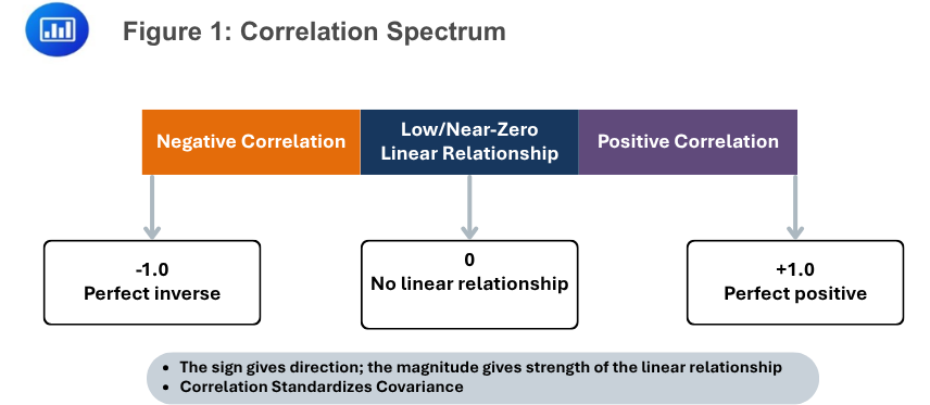
Figure 1 shows the interpretation of the correlation coefficient. The sign tells us direction, while the magnitude tells us strength. The closer the coefficient is to +1 or -1, the tighter the linear relationship. A value near zero does not necessarily mean the variables are unrelated in every possible way; it means they have little or no linear relationship.

$$ \textbf{Table 1: Interpreting Covariance and Correlation} \\
\begin{array}{l|l|l|l}
\textbf{Statistic} & \textbf{Scale} & \textbf{Main Interpretation} & \textbf{Common Trap} \\ \hline
\text{Covariance} & \text{Depends on units} & \text{Direction of co-movement} & \begin{array}{l} \text{Treating a large number} \\ \text{as strong without} \\ \text{considering scale} \end{array} \\ \hline
\text{Correlation} & \text{Ranges from -1 to +1} & \begin{array}{l} \text{Direction and strength of} \\ \text{a linear relationship} \end{array} & \begin{array}{l} \text{Treating correlation as} \\ \text{evidence of causation} \end{array} \\ \hline
\text{Positive value} & \begin{array}{l} \text{Above-mean values tend} \\ \text{to occur together} \end{array} & \begin{array}{l} \text{Same-direction} \\ \text{co-movement} \end{array} & \begin{array}{l} \text{Assuming diversification} \\ \text{is impossible} \end{array} \\ \hline
\text{Negative value} & \begin{array}{l} \text{One variable tends to be} \\ \text{above its mean when the} \\ \text{other is below its mean} \end{array} & \begin{array}{l} \text{Opposite-direction} \\ \text{co-movement} \end{array} & \begin{array}{l} \text{Assuming the relationship} \\ \text{will hold in every future} \\ \text{period} \end{array} \\ \hline
\text{Zero or near zero} & \begin{array}{l} \text{Little average linear} \\ \text{co-movement} \end{array} & \begin{array}{l} \text{Potential diversification} \\ \text{benefit} \end{array} & \begin{array}{l} \text{Ignoring possible} \\ \text{nonlinear relationships} \end{array} \\
\end{array}
$$

Table 1 is a useful way to separate the two statistics. Covariance is the building block in portfolio variance, but correlation is easier to interpret because it is standardized.

Example 2: Calculating and Interpreting Correlation

Suppose we want to convert the covariance from Example 1 into a sample correlation. The sample covariance between the technology fund and cybersecurity fund is 0.001367. The sample standard deviations are 4.69% and 3.10%, respectively.

Solution

Recall that:

$$
r_{X,Y} = \frac{s_{X,Y}}{s_X s_Y}
$$

Where:

• \(r_{X,Y}\) is the sample correlation between the two fund returns
• \(s_{X,Y} = 0.001367\), the sample covariance between the fund returns
• \(s_X = 4.69\%\), the sample standard deviation of the technology fund
• \(s_Y = 3.10\%\), the sample standard deviation of the cybersecurity fund

Use decimal returns for the standard deviations:

$$
r_{X,Y} = \frac{0.001367}{(0.0469)(0.0310)} = 0.94
$$

The sample correlation is approximately 0.94. The two funds show a strong positive linear relationship in this sample. That does not mean one fund caused the other to move. It means their monthly returns moved together closely over the observed period.

Scatter Plots and Linear Relationships

Scatter plots are useful because they show the shape of the relationship behind the correlation number. A tight upward pattern is consistent with positive correlation. A tight downward pattern is consistent with negative correlation. A cloud with no visible slope is consistent with a low or near-zero correlation.

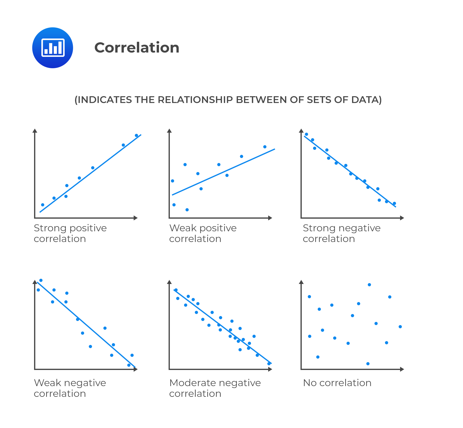
The figure above shows why a visual check helps. Correlation summarizes the direction and strength of a linear relationship, but a scatter plot can reveal outliers, clusters, nonlinearity, or changing regimes. These patterns matter in finance because relationships among returns can change during crises, periods of high inflation, policy surprises, or liquidity stress.

Correlation, Diversification, and Portfolio Risk

Correlation is central to diversification. Diversification is most powerful when assets have low or negative correlations. If two assets are less than perfectly positively correlated, combining them can reduce portfolio volatility relative to a simple weighted average of their individual volatilities.

The intuition is straightforward. If two assets do not move together perfectly, weakness in one asset may be partly offset by strength, stability, or a smaller decline in the other. This is why a portfolio can have lower risk than its individual holdings might suggest when viewed separately.

However, low historical correlation is not a guarantee of future protection. Correlations often rise during market stress. Assets that appeared only loosely related during calm periods may fall together when investors are forced to reduce risk, liquidity becomes scarce, or macroeconomic shocks dominate security-specific factors.

Example 3: Evaluating Diversification Using Correlation

Suppose an equity analyst is considering two potential additions to an existing equity portfolio. The estimated correlations with the current portfolio are shown below.

$$
\begin{array}{l|c}
\textbf{Candidate Asset} & {\textbf{Correlation With Existing} \\ \textbf{Equity Portfolio}} \\ \hline
\text{Global listed infrastructure} & 0.72 \\ \hline
\text{Short-duration government bonds} & -0.18 \\
\end{array}
$$

Based on the correlation values, evaluate which asset is more likely to provide diversification benefits.

Solution

We can start by quoting the interpretation range:

$$
-1 \le \rho_{X,Y} \le 1
$$

Where:

• \(\rho_{X,Y}\) is the correlation between two asset returns
• \(- 1\) indicates a perfect inverse linear relationship
• \(0\) indicates no linear relationship
• \(+ 1\) indicates a perfect positive linear relationship

The short-duration government bond allocation has a correlation of -0.18 with the equity portfolio. This suggests mild opposite-direction co-movement. The listed infrastructure allocation shows a correlation of 0.72 with equities, suggesting a fairly strong positive relationship.

The short-duration government bond allocation is therefore more likely to provide diversification against movements in the equity portfolio. This conclusion is based on correlation alone. A full portfolio decision would also consider expected return, volatility, liquidity, valuation, taxes, and the possibility that correlations change in stress periods.

Excess Returns and Benchmark Relationships

Correlation is often applied to excess returns, which are returns above a risk-free rate or benchmark. The correlation between an asset’s excess return and a benchmark’s excess return helps indicate how closely the asset behaves like the benchmark after adjusting for the common risk-free component.

A high positive correlation with a benchmark suggests that the asset’s active return pattern is closely tied to benchmark movements. That may be expected for a large-cap stock relative to its domestic equity market. A low correlation may suggest that the asset behaves differently from the benchmark, which can matter for active risk, diversification, and performance attribution.

The correlation formula is the same:

$$
\rho_{X,Y} = \frac{\sigma_{X,Y}}{\sigma_X \sigma_Y}
$$

Where:

• \(X\) is the asset’s excess return series
• \(Y\) is the benchmark’s excess return series
• \(\sigma_{X,Y}\) is the covariance between the two excess return series
• \(\sigma_X\) is the standard deviation of the asset’s excess returns
• \(\sigma_Y\) is the standard deviation of the benchmark’s excess returns

When comparing an active manager to a benchmark, correlation should not be interpreted in isolation. A high correlation may simply mean the manager takes broad market exposure. It does not, by itself, prove skill. A low correlation may indicate differentiated positioning, but it may also reflect benchmark mismatch or unintended risk.

Problems in Interpreting Correlation

Correlation is powerful but easy to misuse. Four issues deserve special care.

First, correlation does not imply causation. A positive correlation between two variables does not mean one caused the other. It may reflect a common driver, such as interest rates, inflation expectations, commodity prices, or broad investor risk appetite.

Second, correlation measures linear relationships. Two variables may have a strong nonlinear relationship while still having a low linear correlation. This is especially relevant when payoffs are option-like, capped, floored, or asymmetric.

Third, correlation can be distorted by outliers. A single crisis month or data error can materially change the estimated correlation, especially in small samples.

Fourth, correlation can be unstable over time. Asset relationships often shift across regimes. Equity-bond correlations, for example, may be low or negative in one inflation environment and positive in another. That is why correlation estimates should be evaluated alongside economic reasoning and not treated as fixed constants.

$$ \textbf{Table 2: Correlation Interpretation Checklist} \\
\begin{array}{l|l}
\textbf{Question} & \textbf{Why It Matters} \\ \hline
\text{Is the sign positive, negative, or near zero?} & \text{Identifies the direction of average linear co-movement} \\ \hline
\text{Is the magnitude close to 1 or close to 0?} & \text{Indicates strength of the linear relationship} \\ \hline
\text{Is the sample long and representative?} & \text{Reduces the risk of drawing conclusions from noise} \\ \hline
\text{Are there outliers or crisis observations?} & \text{Helps judge whether the estimate is distorted} \\ \hline
\text{Is the relationship economically plausible?} & \text{Guards against spurious correlation} \\ \hline
\text{Could the relationship be nonlinear?} & \text{Prevents overreliance on a linear statistic} \\
\end{array}
$$

Table 2 should be used as a discipline. A correlation estimate is a starting point for analysis, not the final investment conclusion.

Example 4: Identifying Misinterpretation of Correlation

Suppose an analyst reports that monthly changes in a clean‑energy index and monthly changes in lithium prices have exhibited a correlation of 0.58 over the past five years. The analyst concludes that rising lithium prices caused the clean‑energy index to rise.

Evaluate the validity of this statement.

Solution

The correlation of 0.58 indicates a moderate positive linear association. It does not establish causation. The two series may be connected through common drivers such as global battery demand, electric-vehicle adoption expectations, financing conditions, or investor risk appetite. A stronger research design would be needed before making a causal claim.

The correct interpretation is that the two series tended to move in the same direction over the sample period. The causal conclusion goes beyond what correlation can support.

Interpretation and Evaluation

Several practical principles follow:

• Positive covariance indicates same-direction co-movement relative to the variables’ own means.
• Negative covariance indicates opposite-direction co-movement relative to the variables’ own means.
• Covariance is not standardized, so its magnitude is difficult to compare across datasets.
• Correlation standardizes covariance and ranges from -1 to +1.
• Correlation measures the strength and direction of a linear relationship.
• Correlation does not imply causation.
• Correlation can be distorted by outliers, nonlinearity, small samples, and changing regimes.
• Low or negative correlation can improve diversification, but historical correlation is not a guarantee of future protection.

Question

An analyst observes the following sample statistics for two monthly return series:

$$
\begin{array}{l|c}
\textbf{Statistic} & \textbf{Value} \\ \hline
\text{Sample covariance, } s_{X,Y} & 0.00072 \\ \hline
\text{Sample standard deviation of } X, s_X & 4.0\% \\ \hline
\text{Sample standard deviation of } Y, s_Y & 6.0\% \\
\end{array}
$$

The sample correlation between the two return series is closest to:

1. 0.18
2. 0.30
3. 0.72

Answer Explanation

The correct answer is B.

Recall the correlation formula:

$$
r_{X,Y} = \frac{s_{X,Y}}{s_X s_Y}
$$

Where:

• \(r_{X,Y}\) is the sample correlation between return series \(X\) and \(Y\)
• \(s_{X,Y} = 0.00072\), the sample covariance between the two return series
• \(s_X = 4.0\% = 0.040\), the sample standard deviation of return series \(X\)
• \(s_Y = 6.0\% = 0.060\), the sample standard deviation of return series \(Y\)

Substituting the values:

$$
r_{X,Y} = \frac{0.00072}{(0.040)(0.060)} = \frac{0.00072}{0.00240} = 0.30
$$

The sample correlation is 0.30, indicating a positive but not especially strong linear relationship between the two monthly return series.