Skewness and Kurtosis in Asset Returns: Interpreting Asymmetry and Tail Risk

Why Shape Matters

Mean and standard deviation are powerful, but they are not enough. Two investment strategies can have the same average return and the same volatility while exposing investors to very different experiences. One strategy may have many small gains and occasional sharp losses. Another may have many small losses and occasional large gains. A third may look calm for months and then produce extreme results in both directions.

This learning outcome focuses on the shape of a return distribution. Shape matters because investment risk is not only about how widely returns vary around the mean. It is also about which side of the distribution carries the extreme outcomes and how frequently large deviations occur.

Skewness and kurtosis are the third and fourth statistical moments. They extend the analysis beyond central tendency and dispersion:

• The first moment describes central location, usually the mean.
• The second moment describes dispersion, usually variance.
• The third moment describes asymmetry, or skewness.
• The fourth moment describes tail weight, or kurtosis.

A candidate should be comfortable reading a distribution summary and saying, in clear finance language, what it implies for return behavior, downside risk, upside optionality, and the reliability of models that assume normality.

Skewness: The Direction of Asymmetry

Skewness measures whether a distribution is symmetric or pulled more strongly to one side. A distribution with zero skewness is symmetric. A distribution with positive skewness has a longer or fatter right tail. A distribution with negative skewness has a longer or fatter left tail.

The sample skewness measure is commonly approximated as:

$$
\text{Skew}(X) = \frac{1}{n} \sum_{i=1}^{n} \left( \frac{X_i – \bar{X}}{s} \right)^3
$$

Where:

• \(\text{Skew}(X)\) is the skewness of the return series
• \(n\) is the number of observations
• \(X_i\) is observation \(i\)
• \(\bar{X}\) is the sample mean
• \(s\) is the sample standard deviation
• \(\left( \frac{X_i – \bar{X}}{s} \right)^3\) is the cubed standardized deviation from the mean

The cubing is important. Positive deviations remain positive, and negative deviations remain negative. Large observations far from the mean receive greater weight than small observations near the mean. Because each deviation is divided by the standard deviation, skewness is scale-free. It can be compared across return series measured in different units or magnitudes.

Figure 1: Skewness and Tail Direction

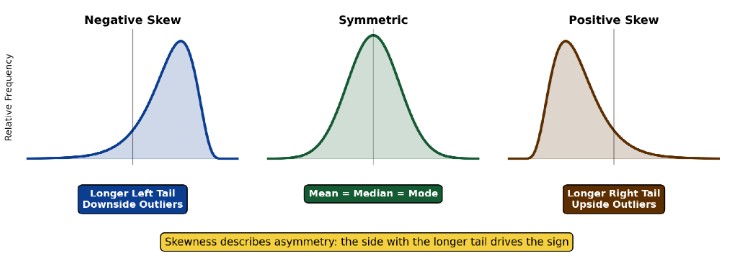
Figure 1 shows the key interpretation. A negatively skewed return distribution has a longer left tail, which suggests greater exposure to unusually poor returns. A positively skewed dFistribution has a longer right tail, which suggests greater exposure to unusually strong returns. A symmetric distribution has balanced tails, so the mean, median, and mode are typically close or equal.

Mean, Median, and Mode in Skewed Distributions

The relationship among the mean, median, and mode provides a useful visual clue about skewness:

$$ \textbf{Table 1: Skewness and Measures of Central Tendency} \\
\begin{array}{l|c|c|c}
{\textbf{Distribution} \\ \text{Shape}} & \textbf{Tail Direction} & \textbf{Common Relationship} & \textbf{Return Interpretation} \\ \hline
\text{Symmetric} & \text{Balanced tails} & \text{Mean} = \text{Median} = \text{Mode} & {\text{Positive and negative} \\ \text{deviations are} \\ \text{broadly balanced}} \\ \hline
{\text{Positively} \\ \text{skewed}} & \text{Longer right tail} & \text{Mean} > \text{Median} > \text{Mode} & {\text{Occasional large} \\ \text{gains may pull} \\ \text{the mean upward}} \\ \hline
{\text{Negatively} \\ \text{skewed}} & \text{Longer left tail} & \text{Mean} < \text{Median} < \text{Mode} & {\text{Occasional large} \\ \text{losses may pull} \\ \text{the mean downward}} \\ \end{array} $$

Table 1 is useful in exam questions that provide summary statistics. If the mean is materially less than the median, the analyst should consider the possibility of negative skew. If the mean is materially greater than the median, positive skew may be present. The relationship is not a substitute for a formal skewness calculation, but it is a practical diagnostic.

Interpreting Skewness in Investment Work

In investment analysis, skewness is closely linked to the character of tail risk.

A negatively skewed strategy may look attractive for long periods because it earns many small positive returns. The concern is that it may occasionally suffer a large loss. Strategies involving short volatility exposure, leveraged carry trades, illiquid credit, or concentrated private investments can sometimes display this pattern. Negative skewness is not automatically unacceptable, but it should usually command careful risk controls and an adequate expected return premium.

A positively skewed strategy may experience many small losses or modest results but preserve the chance of a large gain. Certain venture-capital, trend-following, commodity, or option-like strategies may display positive skewness. Positive skewness can be attractive because the upside tail may be valuable, but it does not eliminate the need to evaluate dispersion, drawdowns, and the probability of loss.

A zero-skewness return distribution is symmetric, but symmetry alone does not make an investment safe. The tails may still be heavy, which is why kurtosis must be considered alongside skewness.

Example 1: Interpreting Negative Skewness

Suppose we want to evaluate the shape of monthly returns for a private credit fund that provides short-term financing to middle-market companies. A risk system reports the following summary statistics:

$$
\begin{array}{l|c}
\textbf{Statistic} & \textbf{Value} \\ \hline
\text{Mean monthly return} & 0.62\% \\ \hline
\text{Median monthly return} & 0.74\% \\ \hline
\text{Sample standard deviation} & 1.85\% \\ \hline
\text{Skewness} & -1.10 \\
\end{array}
$$

The objective is to interpret the reported skewness and explain the investment implication. We proceed as follows:

Recall that:

$$
\text{Skew}(X) = \frac{1}{n} \sum_{i=1}^{n} \left( \frac{X_i – \bar{X}}{s} \right)^3
$$

Where:

• \(X_i\) is the monthly return in month \(i\)
• \(\bar{X}\) is the sample mean monthly return
• \(s\) is the sample standard deviation of monthly returns
• \(n\) is the number of monthly return observations
• \(\text{Skew}(X) = -1.10\) is the reported skewness

Because the skewness is negative, the return distribution is left-skewed. The left tail is longer or fatter than the right tail. The mean is also lower than the median, which is consistent with negative outliers pulling the average downward.

The interpretation is that the fund may experience many stable or mildly positive months, but it is exposed to occasional poor months. For performance evaluation, the analyst should not rely only on the positive average return. The negative skewness points to downside tail risk that may be especially relevant during credit stress, liquidity pressure, or borrower default clusters.

Kurtosis: The Weight of the Tails

Kurtosis measures the weight of a distribution’s tails relative to the rest of the distribution. In finance, the most important interpretation is not simply whether the center of the distribution appears tall. The key issue is whether the distribution produces extreme outcomes more or less frequently than a normal distribution.

A normal distribution has kurtosis of 3. Analysts often use excess kurtosis, which is kurtosis minus 3. Under this convention, a normal distribution has excess kurtosis of 0.

For a sufficiently large sample, excess kurtosis can be approximated as:

$$
\text{Kurt}_E(X) = \frac{1}{n} \sum_{i=1}^{n} \left( \frac{X_i – \bar{X}}{s} \right)^4 – 3
$$

Where:

• \(\text{Kurt}_E(X)\) is the excess kurtosis of the return series
• \(n\) is the number of observations
• \(X_i\) is observation \(i\)
• \(\bar{X}\) is the sample mean
• \(s\) is the sample standard deviation
• \(\left( \frac{X_i – \bar{X}}{s} \right)^4\) is the fourth power of the standardized deviation from the mean
• \(3\) is subtracted so that the normal distribution has excess kurtosis of zero

The relationship between kurtosis and excess kurtosis is:

$$
\text{Kurt}(X) = \text{Kurt}_E(X) + 3
$$

Where:

• \(\text{Kurt}(X)\) is kurtosis
• \(\text{Kurt}_E(X)\) is excess kurtosis
• \(3\) is the kurtosis of a normal distribution

Like skewness, kurtosis is scale-free. It can be compared across return series even when the returns are measured in different units.

Leptokurtic, Mesokurtic, and Platykurtic Distributions

Figure 2: Kurtosis and Tail Weight

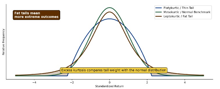
Figure 2 highlights the practical meaning of kurtosis. A leptokurtic distribution has heavier tails than the normal distribution, so extreme outcomes are more frequent than a normal model would suggest. A mesokurtic distribution has tail behavior similar to the normal distribution. A platykurtic distribution has thinner tails and fewer extreme outcomes than the normal benchmark.

$$ \textbf{Table 2: Types of Kurtosis} \\
\begin{array}{l|c|c|c}
\textbf{Distribution Type} & \textbf{Kurtosis} & \textbf{Excess Kurtosis} & \textbf{Tail Interpretation} \\ \hline
\text{Platykurtic} & \text{Less than 3} & \text{Less than 0} & {\text{Thinner tails than the} \\ \text{normal distribution}} \\ \hline
\text{Mesokurtic} & \text{Equal to 3} & \text{Equal to 0} & {\text{Similar tail weight to} \\ \text{the normal distribution}} \\ \hline
\text{Leptokurtic} & \text{Greater than 3} & \text{Greater than 0} & {\text{Fatter tails than the} \\ \text{normal distribution}} \\
\end{array}
$$

Table 2 is one of the most important interpretation tools in this learning outcome. Many financial return distributions are leptokurtic. This means a normal model may underestimate the probability of very large gains or losses, especially during periods of market stress.

Example 2: Distinguishing Kurtosis from Excess Kurtosis

Suppose we want to evaluate monthly returns for a global macro fund. One risk report states that the fund’s kurtosis is 4.60, while another report states that its excess kurtosis is 1.60. A junior analyst thinks the two systems disagree.

Solution

We know that:

$$
\text{Kurt}(X) = \text{Kurt}_E(X) + 3
$$

Where:

• \(\text{Kurt}(X) = 4.60\) is the reported kurtosis
• \(\text{Kurt}_E(X)\) is the reported excess kurtosis
• \(3\) is the kurtosis of a normal distribution

Solving for excess kurtosis:

$$
\text{Kurt}_E(X) = 4.60 – 3 = 1.60
$$

The two reports do not disagree. They are using different reporting conventions. The distribution is leptokurtic because kurtosis is greater than 3 and excess kurtosis is greater than 0. The fund’s return distribution therefore has heavier tails than a normal distribution.

The practical implication is that a model assuming normality may underestimate the likelihood of extreme monthly returns. That risk could appear on either side of the distribution, so kurtosis should be interpreted together with skewness to understand whether the more concerning tail is primarily downside or upside.

Combining Skewness and Kurtosis

Skewness and kurtosis should be interpreted together. Skewness tells the analyst whether the distribution is asymmetric and which side has the longer tail. Kurtosis tells the analyst whether extreme observations are more common than under the normal benchmark.

$$ \textbf{Table 3: Interpreting Skewness and Excess Kurtosis Together} \\
\begin{array}{l|c|c}
\textbf{Skewness} & \textbf{Excess Kurtosis} & \textbf{Likely Interpretation} \\ \hline
\text{Near 0} & \text{Near 0} & {\text{Approximately symmetric} \\ \text{with normal-like tails}} \\ \hline
\text{Positive} & \text{Positive} & {\text{Upside tail is important,} \\ \text{and extreme outcomes are} \\ \text{more frequent than normal}} \\ \hline
\text{Negative} & \text{Positive} & {\text{Downside tail is important,} \\ \text{and extreme outcomes are} \\ \text{more frequent than normal}} \\ \hline
{\text{Positive or} \\ \text{negative}} & \text{Negative} & {\text{Asymmetry may exist, but} \\ \text{tails are thinner than normal}} \\
\end{array}
$$

Table 3 matters because an analyst can draw the wrong conclusion by looking at only one statistic. Positive excess kurtosis alone tells us that the tails are heavy, but it does not identify which tail is more important. Negative skewness alone tells us that the left tail is longer, but it does not tell us whether both tails are unusually heavy compared with a normal distribution.

Example 3: Evaluating an Asset Return Distribution

Suppose we wish to evaluate whether a normal distribution is a reasonable first approximation for monthly returns of an emerging-market equity strategy. A summary report provides the following statistics:

$$
\begin{array}{l|r}
\textbf{Statistic} & \textbf{Value} \\ \hline
\text{Mean monthly return} & 0.95\% \\ \hline
\text{Median monthly return} & 1.30\% \\ \hline
\text{Sample standard deviation} & 6.40\% \\ \hline
\text{Skewness} & -0.80 \\ \hline
\text{Excess kurtosis} & 2.22 \\
\end{array}
$$

The objective is to interpret the shape of the distribution and evaluate whether normality is likely to be a strong modeling assumption.

Solution

The negative skewness indicates a left-skewed distribution. The mean is also below the median, which is consistent with negative outliers pulling the mean downward.

The positive excess kurtosis indicates a leptokurtic distribution with fatter tails than the normal distribution. Combining the two statistics, the strategy appears exposed to downside tail risk and more frequent extreme outcomes than a normal model would imply.

A normal distribution is therefore not a strong modeling assumption for stress testing. It may understate the probability of sharp negative months. A more careful analysis would examine drawdowns, tail percentiles, stress periods, and whether the return process changes across market regimes.

Practical Evaluation Issues

Skewness and kurtosis are powerful, but they should be evaluated with care.

First, they are sample estimates. A small sample may produce unstable skewness and kurtosis estimates. One or two observations can change the result materially. This is especially important in private-market, hedge fund, and new-strategy datasets that may have limited return history.

Second, the analyst must know whether a system reports kurtosis or excess kurtosis. A value of 3 may mean normal-like tails if the statistic is kurtosis. The same value would mean very fat tails if the statistic is excess kurtosis.

Third, the statistics should be interpreted alongside histograms, box-and-whisker plots, drawdowns, and scenario analysis. A single number is useful, but a visual distribution can reveal clustering, outliers, regime shifts, or data errors.

Fourth, financial return distributions are often not stationary. Volatility, skewness, and tail behavior can change across market regimes. A strategy that looked symmetric during a low-volatility period may become negatively skewed during a liquidity shock.

Finally, scale-free does not mean risk-free. Skewness and kurtosis are dimensionless, but they still describe meaningful economic risk. A strategy with negative skewness and high positive excess kurtosis can carry severe downside risk even when its average return appears attractive.

Interpretation and Evaluation

Several practical principles follow:

• Skewness measures asymmetry
• Positive skewness means the right tail is longer or fatter
• Negative skewness means the left tail is longer or fatter
• Normal distributions have skewness of zero
• Kurtosis measures tail weight relative to the rest of the distribution
• A normal distribution has kurtosis of 3 and excess kurtosis of zero
• Positive excess kurtosis indicates fat tails and more frequent extreme outcomes than normal
• Negative excess kurtosis indicates thin tails and fewer extreme outcomes than normal
• Skewness identifies tail direction; kurtosis identifies tail weight
• Many financial return distributions are not normal, especially during stress periods

Question

An analyst summarizes monthly returns for a battery-metals equity strategy as follows:

$$
\begin{array}{l|c}
\textbf{Statistic} & \textbf{Value} \\ \hline
\text{Mean monthly return} & 1.10\% \\ \hline
\text{Median monthly return} & 1.80\% \\ \hline
\text{Standard deviation} & 8.60\% \\ \hline
\text{Skewness} & -0.92 \\ \hline
\text{Excess kurtosis} & 1.75 \\
\end{array}
$$

The most appropriate interpretation is that the return distribution is:

1. approximately normal because the average return is positive.
2. left-skewed and fat-tailed relative to a normal distribution.
3. right-skewed and thin-tailed relative to a normal distribution.

The correct answer is B.

A normal distribution has skewness of zero and excess kurtosis of zero. The strategy’s skewness is -0.92, indicating a left-skewed distribution. The left tail is longer or fatter than the right tail, which means negative outliers are an important part of the return behavior.

The strategy’s excess kurtosis is 1.75, which is positive. This indicates a leptokurtic, or fat-tailed, distribution relative to the normal distribution. Extreme outcomes are more frequent than a normal model would suggest.

The fact that the mean return is positive does not make the distribution normal. In fact, the mean is below the median, which is consistent with negative outliers pulling the mean downward.

A is incorrect because a positive mean does not imply normality. The reported skewness and excess kurtosis both indicate non-normal return behavior.

C is incorrect because the skewness is negative, not positive, and the excess kurtosis is positive, not negative. The distribution is left-skewed and fat-tailed, not right-skewed and thin-tailed.