Semi-Deviation and Coefficient of Variation: Downside Risk and Risk per Unit of Return

Why Additional Dispersion Measures Are Needed

Standard deviation is the most familiar measure of volatility, but it treats upside and downside variability symmetrically. A return that is far above the mean increases standard deviation just as much as a return that is far below the mean. That treatment is mathematically useful, but it is not always aligned with how investors experience risk.

Many investors are especially concerned with downside risk. A pension fund may care about returns falling below the rate needed to meet benefit obligations. A foundation may care about returns falling below its spending rate. A risk manager may care more about shortfalls below a benchmark than about unusually strong positive returns. In such cases, semi-deviation and target downside deviation can be more informative than ordinary standard deviation.

The coefficient of variation answers a different question. It compares dispersion with the mean. This makes it useful when two investments have different average returns and the analyst wants to understand risk per unit of return.

Semi-Variance and Semi-Deviation

Semi-variance measures the average squared deviation of observations that fall below a chosen reference point. When the reference point is the mean, semi-variance focuses on observations below the mean. Semi-deviation is the square root of semi-variance.

This distinction matters. Variance and standard deviation treat upside and downside surprises equally. Semi-variance and semi-deviation focus only on the unfavorable side of the distribution.

The semi-variance below the sample mean can be written as:

$$
s_{\text{semi}}^2 = \frac{\sum_{X_i < \bar{X}} \left(X_i – \bar{X}\right)^2}{n-1} $$

Where:

• \(s_{\text{semi}}^2\) is the sample semi-variance below the sample mean
• \(X_i\) is observation \(i\)
• \(\bar{X}\) is the sample mean
• \(n\) is the total number of observations in the sample
• \(n – 1\) is the sample degrees of freedom

The semi-deviation is:

$$
s_{\text{semi}} = \sqrt{s_{\text{semi}}^2}
$$

Where:

• \(s_{\text{semi}}\) is the sample semi-deviation
• \(s_{\text{semi}}^2\) is the sample semi-variance

The denominator is based on the total sample size adjustment rather than only the number of observations below the mean. The reason is that the statistic is being estimated from the full return sample, even though only the negative deviations contribute to the numerator.

Figure 1: Downside-Risk Focus of Semi-Deviation

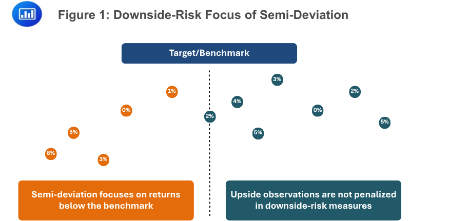
Figure 1 shows the logic behind semi-deviation. Returns below the target or benchmark are treated as unfavorable deviations. Returns above the target are not penalized by the downside-risk measure. This does not mean upside returns are irrelevant to the investment decision. It means the statistic has been designed to isolate shortfall risk.

Example 1: Calculating Semi-Deviation Below the Mean

Suppose a factor portfolio has recorded the following annual returns over five years:

$$
\begin{array}{c|c}
\textbf{Year} & \textbf{Return} \\ \hline
1 & -6.0\% \\ \hline
2 & -1.0\% \\ \hline
3 & 3.0\% \\ \hline
4 & 5.0\% \\ \hline
5 & 9.0\% \\
\end{array}
$$

Calculate the semi‑deviation of returns below the sample mean.

Solution

Recall:

$$
s_{\text{semi}}^2 = \frac{\sum_{X_i < \bar{X}} \left(X_i – \bar{X}\right)^2}{n-1} $$

Where:

• \(s_{\text{semi}}^2\) is the sample semi-variance below the sample mean
• \(X_i\) is the annual return in year \(i\)
• \(\bar{X}\) is the sample mean annual return
• \(n = 5\), the number of annual returns
• \(n – 1 = 4\), the sample degrees of freedom

First calculate the sample mean:

$$
\bar{X} = \frac{-6\% – 1\% + 3\% + 5\% + 9\%}{5} = 2.0\%
$$

The observations below the mean are -6.0% and -1.0%. Their deviations from the mean are:

$$
\begin{array}{c|c|c}
\textbf{Return Below Mean} & \textbf{Deviation From Mean} & \textbf{Squared Deviation} \\ \hline
-6.0\% & -8.0\% & 0.0064 \\ \hline
-1.0\% & -3.0\% & 0.0009 \\ \hline
\textbf{Total} & & 0.0073 \\
\end{array}
$$

The sample semi-variance is:

$$
s_{\text{semi}}^2 = \frac{0.0073}{4} = 0.001825
$$

Now quote the semi-deviation formula:

$$
s_{\text{semi}} = \sqrt{s_{\text{semi}}^2}
$$

Where:

• \(s_{\text{semi}}\) is the sample semi-deviation
• \(s_{\text{semi}}^2 = 0.001825\), the sample semi-variance

The sample semi-deviation is:

$$
s_{\text{semi}} = \sqrt{0.001825} = 4.27\%
$$

The semi-deviation is 4.27%. It measures downside dispersion below the mean return of 2.0%. The positive returns above the mean do not increase the numerator because the statistic is designed to focus on downside variation.

Target Downside Deviation

In many investment problems, the relevant reference point is not the mean. The investor may have a target return, benchmark return, required return, or minimum acceptable return. Target downside deviation, also called target semi-deviation, measures dispersion of observations that fall below that chosen target.

The sample target downside deviation is:

$$
s_{\text{Target}} = \sqrt{\frac{\sum_{X_i \le B} \left(X_i – B\right)^2}{n-1}}
$$

Where:

• \(s_{\text{Target}}\) is the sample target downside deviation
• \(X_i\) is observation \(i\)
• \(B\) is the target return, benchmark, or minimum acceptable return
• \(n\) is the total number of sample observations
• \(n – 1\) is the sample degrees of freedom
• The summation includes observations at or below the target

If an observation equals the target, its deviation is zero. Including it does not change the numerator, but it is still part of the full sample size. A higher target normally increases target downside deviation because more observations fall below the target and the shortfall amounts become larger.

Example 2: Calculating Target Downside Deviation

Suppose a monthly‑return strategy produced the following results over a 12‑month period.

$$
\begin{array}{c|c}
\textbf{Month} & \textbf{Return} \\ \hline
1 & 5.0\% \\ \hline
2 & 4.0\% \\ \hline
3 & -2.0\% \\ \hline
4 & 1.0\% \\ \hline
5 & 3.0\% \\ \hline
6 & -1.0\% \\ \hline
7 & 6.0\% \\ \hline
8 & 2.0\% \\ \hline
9 & 0.0\% \\ \hline
10 & 4.0\% \\ \hline
11 & -3.0\% \\ \hline
12 & 5.0\% \\
\end{array}
$$

If the target return is 2.0% per month, calculate the downside semi‑deviation of the strategy’s returns relative to the 2.0% target.

Solution

We know that:

$$
s_{\text{Target}} = \sqrt{\frac{\sum_{X_i \le B} \left(X_i – B\right)^2}{n-1}}
$$

Where:

• \(s_{\text{Target}}\) is the sample target downside deviation
• \(X_i\) is the return in month \(i\)
• \(B = 2.0\%\), the monthly target return
• \(n = 12\), the number of monthly observations
• \(n – 1 = 11\), the sample degrees of freedom

Now identify the observations below the target and calculate squared shortfalls:

$$
\begin{array}{c|c|c}
\textbf{Return at or Below Target} & \textbf{Deviation From 2.0% Target} & \textbf{Squared Deviation} \\ \hline
-2.0\% & -4.0\% & 0.0016 \\ \hline
1.0\% & -1.0\% & 0.0001 \\ \hline
-1.0\% & -3.0\% & 0.0009 \\ \hline
2.0\% & 0.0\% & 0.0000 \\ \hline
0.0\% & -2.0\% & 0.0004 \\ \hline
-3.0\% & -5.0\% & 0.0025 \\ \hline
\textbf{Total} & & 0.0055 \\
\end{array}
$$

The target downside deviation is:

$$
s_{\text{Target}} = \sqrt{\frac{0.0055}{11}} = 2.24\%
$$

The strategy’s sample target downside deviation is 2.24%. This figure summarizes the downside dispersion relative to the 2.0% target. The months with returns above 2.0% are not treated as unfavorable in this statistic.

How the Target Affects Downside Deviation

The target is not a minor detail. It determines which observations are treated as shortfalls and how large the shortfalls are. A higher target usually increases the target downside deviation because more observations fall below the threshold.

$$ \textbf{Table 1: Effect of Raising the Target Return} \\
\begin{array}{l|l|l}
\textbf{Target Return} & {\textbf{Observations Treated} \\ \textbf{as Shortfalls}} & {\textbf{General Effect on Target} \\ \textbf{Downside Deviation}} \\ \hline
\text{Low target} & \text{Fewer observations} & \text{Lower downside deviation} \\ \hline
\text{Moderate target} & \text{More observations} & \text{Higher downside deviation} \\ \hline
\text{High target} & \text{Many observations} & \text{Highest downside deviation} \\
\end{array}
$$

Table 1 is useful for interpretation. A manager may appear to have modest downside risk relative to a 0% target but much larger downside risk relative to a 6% required return. The statistic must therefore be interpreted together with the target used.

Example 3: Evaluating a Higher Target

Suppose we want to evaluate the same strategy from Example 2, but the investor raises the monthly target from 2.0% to 4.0%. Determine whether the target downside deviation is likely to increase or decrease, and explain why.

Solution

$$
s_{\text{Target}} = \sqrt{\frac{\sum_{X_i \le B} \left(X_i – B\right)^2}{n-1}}
$$

Where:

• \(s_{\text{Target}}\) is the sample target downside deviation
• \(B\) is the target return
• \(X_i\) is the return in month \(i\)
• \(n\) is the total number of monthly observations

Raising the target from 2.0% to 4.0% causes more returns to fall at or below the target. It also increases the shortfall for any return already below the previous target. As a result, the target downside deviation should increase.

This is not a flaw in the statistic. It is the point of the statistic. A higher required return makes the same return series look riskier from a shortfall perspective.

Coefficient of Variation

The coefficient of variation measures dispersion relative to the mean. It is useful when comparing investments that have different average returns.

The coefficient of variation is:

$$
CV = \frac{s}{\bar{X}}
$$

Where:

• \(CV\) is the coefficient of variation
• \(s\) is the sample standard deviation
• \(\bar{X}\) is the sample mean

A lower CV indicates less dispersion per unit of mean return. A higher CV indicates more dispersion per unit of mean return. In simple language, CV asks: “How much volatility is the investor taking for each unit of average return?”

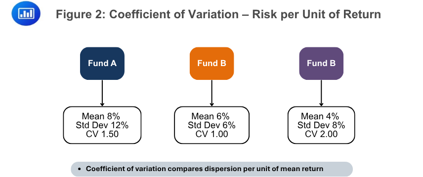
Figure 2 illustrates why the coefficient of variation can change a ranking. Fund A has a higher average return than Fund B, but it also has more volatility. Fund C has the lowest mean and relatively high volatility, producing the largest coefficient of variation. The CV is therefore a scaled measure of risk, not merely a volatility measure.

The CV is especially helpful when expected returns are positive and meaningfully different across assets. It is less useful when the mean is close to zero, and it can become difficult to interpret when the mean is negative. A negative or near-zero mean can produce a misleading or unstable CV.

Example 4: Comparing Investments Using the Coefficient of Variation

Three sector funds have the following sample mean monthly returns and monthly standard deviations:

$$
\begin{array}{l|c|c}
\textbf{Fund} & \textbf{Mean Monthly Return} & \textbf{Monthly Standard Deviation} \\ \hline
\text{Digital Infrastructure} & 1.8\% & 2.7\% \\ \hline
\text{Regulated Utilities} & 1.2\% & 0.9\% \\ \hline
\text{Biotechnology Innovation} & 2.2\% & 5.5\% \\
\end{array}
$$

Calculate the risk per unit of average monthly return for each fund. Identify which fund exhibits the lowest dispersion per unit of mean return and which exhibits the highest.

Solution

$$
CV = \frac{s}{\bar{X}}
$$

Where:

• \(CV\) is the coefficient of variation
• \(s\) is the sample standard deviation of monthly returns
• \(\bar{X}\) is the sample mean monthly return

Now calculate each fund’s CV:

$$
CV_{\text{Digital Infrastructure}} = \frac{2.7\%}{1.8\%} = 1.50
$$

$$
CV_{\text{Regulated Utilities}} = \frac{0.9\%}{1.2\%} = 0.75
$$

$$
CV_{\text{Biotechnology Innovation}} = \frac{5.5\%}{2.2\%} = 2.50
$$

The Regulated Utilities fund has the lowest CV, so it has the lowest dispersion per unit of average monthly return. The Biotechnology Innovation fund has the highest CV, so it has the highest dispersion per unit of average monthly return.

This does not automatically make the utility fund the best investment. The analyst would still consider expected future returns, valuation, liquidity, tax effects, and diversification benefits. The CV is one useful comparison, not the full investment decision.

Semi-Deviation Versus Coefficient of Variation

Semi-deviation and coefficient of variation answer different questions. Semi-deviation focuses on downside variability. Coefficient of variation scales total dispersion relative to the mean.

$$ \textbf{Table 2: Semi-Deviation and Coefficient of Variation Compared} \\
\begin{array}{l|c|c|c}
\textbf{Measure} & \textbf{Main Question Answered} & \textbf{Best Used When} & \textbf{Main Limitation} \\ \hline
\text{Semi-deviation} & \begin{array}{l} \text{How much downside} \\ \text{variability is present?} \end{array} & \begin{array}{l} \text{Investor is especially} \\ \text{concerned with shortfalls} \\ \text{below the mean or target} \end{array} & \text{Ignores upside volatility} \\ \hline
\begin{array}{l} \text{Target downside} \\ \text{deviation} \end{array} & \begin{array}{l} \text{How much shortfall risk} \\ \text{exists relative to a chosen} \\ \text{target?} \end{array} & \begin{array}{l} \text{A benchmark, required} \\ \text{return, or minimum} \\ \text{acceptable return matters} \end{array} & \begin{array}{l} \text{Sensitive to the chosen} \\ \text{target} \end{array} \\ \hline
\text{Coefficient of variation} & \begin{array}{l} \text{How much total} \\ \text{dispersion exists per unit} \\ \text{of mean return?} \end{array} & \begin{array}{l} \text{Comparing investments} \\ \text{with different positive} \\ \text{means} \end{array} & \begin{array}{l} \text{Hard to interpret when} \\ \text{the mean is near zero or} \\ \text{negative} \end{array} \\
\end{array}
$$

Table 2 should prevent a common exam error. Semi-deviation is not “half of standard deviation.” It is a downside-risk statistic. CV is not an absolute risk statistic. It is a relative-dispersion statistic.

Evaluation Issues and Common Traps

Semi-deviation and CV are useful, but both require judgment.

For semi-deviation, the analyst must decide the relevant reference point. A mean-based semi-deviation tells one story; a target-based downside deviation may tell another. A strategy with few losses relative to zero may still have high shortfall risk relative to a 7% required return.

For CV, the mean matters. When the mean is very small, the CV can become extremely large and unstable. When the mean is negative, the sign of CV may be difficult to interpret because the statistic is intended to compare dispersion relative to a positive return base. In such cases, an analyst should consider additional risk measures and the economic context rather than relying on CV alone.

Interpretation and Evaluation

Several practical principles follow:

• Standard deviation treats upside and downside variation symmetrically.
• Semi-deviation focuses on downside variation below the mean.
• Target downside deviation focuses on shortfalls below a selected benchmark or minimum acceptable return.
• A higher target normally increases target downside deviation.
• Coefficient of variation measures dispersion per unit of mean return.
• A lower CV indicates less relative dispersion when mean returns are positive.
• CV is difficult to interpret when the mean is close to zero or negative.
• Semi-deviation and CV should be interpreted with sample size, outliers, and investment objective in mind.

Question

An analyst compares three portfolios using the following monthly return statistics:

$$
\begin{array}{l|c|c}
\textbf{Portfolio} & \textbf{Mean Monthly Return} & \textbf{Monthly Standard Deviation} \\ \hline
\text{A} & 1.5\% & 2.1\% \\ \hline
\text{B} & 2.0\% & 3.8\% \\ \hline
\text{C} & 0.9\% & 1.8\% \\
\end{array}
$$

Based on the coefficient of variation, which portfolio has the lowest relative dispersion?

1. Portfolio A
2. Portfolio B
3. Portfolio C

Answer Explanation

The correct answer is A.

$$
CV = \frac{s}{\bar{X}}
$$

Where:

• \(CV\) is the coefficient of variation
• \(s\) is the sample standard deviation of monthly returns
• \(\bar{X}\) is the sample mean monthly return

Calculate the coefficient of variation for each portfolio:

$$
CV_A = \frac{2.1\%}{1.5\%} = 1.40
$$

$$
CV_B = \frac{3.8\%}{2.0\%} = 1.90
$$

$$
CV_C = \frac{1.8\%}{0.9\%} = 2.00
$$

Portfolio A has the lowest coefficient of variation, so it has the lowest dispersion per unit of mean monthly return.

B is incorrect because Portfolio B has a coefficient of variation of 1.90, which is higher than Portfolio A’s coefficient of variation

C is incorrect because Portfolio C has a coefficient of variation of 2.00, the highest among the three portfolios