Statistical Measures of Asset Returns: Mean, Median, Variance, Standard Deviation, and Dispersion

Why Statistical Characteristics Matter

A return series is rarely understood by looking at a single observation. A portfolio may earn 8% in one year, lose 12% the next year, and then recover sharply. An analyst therefore needs summary measures that describe what is typical, where observations lie, how widely they vary, and whether a few unusual observations are distorting the picture.

This learning outcome focuses on two broad families of measures. The first family describes central tendency and location: mean, median, mode, trimmed mean, winsorized mean, and quantiles. The second family describes dispersion: range, mean absolute deviation, median absolute deviation, variance, standard deviation, and scaled volatility.

These measures are foundational for security analysis, manager evaluation, risk reporting, and portfolio construction. A strong candidate does not merely calculate them. A strong candidate also explains what each statistic reveals, what it hides, and when it may mislead.

Population, Sample, and the Return Dataset

A population is the complete set of observations relevant to the question being asked. A sample is a subset of that population. In finance, we usually work with samples because the full population of possible future returns is not observable.

For example, a dataset of 60 monthly returns for a listed infrastructure fund is a sample from a broader return-generating process. We use that sample to estimate the fund’s typical return and risk. The quality of the estimate depends on the number of observations, the stability of the return process, and the presence of outliers or unusual market events.

A useful statistical summary should therefore always be interpreted in context. The same average return may have very different implications if the sample contains stable monthly returns, pandemic-era market shocks, commodity price jumps, or one-off data errors.

Central Tendency: Mean, Median, and Mode

A measure of central tendency attempts to describe a typical or central value in a dataset. The three basic measures are the mean, median, and mode.

The arithmetic mean is:

\[
\mu = \frac{1}{n} \sum_{i=1}^{n} X_i
\]

Where:

• \( \mu \) is the population mean or arithmetic average
• \( n \) is the number of observations
• \( X_i \) is the value of observation \( i \)

When the data are a sample, the sample mean is commonly written as:

\[
\bar{X} = \frac{1}{n} \sum_{i=1}^{n} X_i
\]

Where:

• \( \bar{X} \) is the sample mean
• \( n \) is the number of sample observations
• \( X_i \) is the value of observation \( i \)

The mean uses every observation, which is both a strength and a weakness. It reflects the full dataset, but it is sensitive to outliers. A single unusually large gain or loss can pull the mean away from the center of most observations.

The median is the middle observation after the data have been sorted. If the number of observations is odd, the median is the middle-ranked value:

\[
\text{Median} = X_{\left(\frac{n+1}{2}\right)}
\]

Where:

• \(\text{Median}\) is the middle value of the ordered dataset
• \(X_{\left(\frac{n+1}{2}\right)}\) is the observation in the middle position
• \(n\) is the number of observations

If the number of observations is even, the median is the average of the two middle observations:

\[
\text{Median} = \frac{X_{\left(\frac{n}{2}\right)} + X_{\left(\frac{n}{2}+1\right)}}{2}
\]

Where:

• \(X_{\left(\frac{n}{2}\right)}\) is the lower middle observation
• \(X_{\left(\frac{n}{2}+1\right)}\) is the upper middle observation
• \(n\) is an even number of observations

The median is more robust than the mean because it depends on position rather than magnitude. Extreme returns can change the mean dramatically while leaving the median almost unchanged.

The mode is the value that occurs most frequently. It is particularly useful when values cluster around one or more points. A dataset may have one mode, multiple modes, or no repeated value at all. In investment data, the modal interval is often more useful than the exact mode because returns are commonly grouped into histogram bins.

$$ \textbf{Table 1: Mean, Median, and Mode Compared} \\
\begin{array}{l|l|l|l}
\textbf{Measure} & \textbf{Main Idea} & \textbf{Strength} & \textbf{Main Weakness} \\ \hline
\text{Mean} & {\text{Average of all} \\ \text{observations}} & \text{Uses all data values} & \text{Sensitive to outliers} \\ \hline
\text{Median} & \text{Middle value after sorting} & {\text{Robust to extreme} \\ \text{observations} } & {\text{Ignores the magnitude of} \\ \text{most observations} }\\ \hline
\text{Mode} & {\text{Most frequent value or} \\ \text{interval}} & \text{Identifies clustering} & {\text{May be absent or may} \\ \text{not be unique}} \\
\end{array}
$$

Table 1 is a useful exam guide. If a question emphasizes an outlier, the median or a robust mean may be more informative than the arithmetic mean. If a question asks for the average using all observations, the mean is usually intended. If the question focuses on clustering, the mode or modal interval may be the relevant statistic.

Example 1: Calculating and Interpreting Measures of Central Tendency

Assume we wish to describe the central tendency of seven monthly returns for a digital payments stock. The returns, sorted from lowest to highest, are:

$$\begin{array}{c|c}
\textbf{Month} & \textbf{Return} \\ \hline
1 & -18.0\% \\ \hline
2 & -2.0\% \\ \hline
3 & 1.0\% \\ \hline
4 & 2.0\% \\ \hline
5 & 3.0\% \\ \hline
6 & 4.0\% \\ \hline
7 & 5.0\% \\
\end{array}
$$

The objective is to calculate the mean and median and explain which statistic better describes the typical month.

Solution

The mean formula is given by:

$$
\bar{X} = \frac{1}{n} \sum_{i=1}^{n} X_i
$$

Where:

• \(\bar{X}\) is the sample mean return
• \(n = 7\), the number of monthly returns
• \(X_i\) is the return in month \(i\)

Substitute the returns:

$$ \begin{align*}
\bar{X} & = \frac{-18\% – 2\% + 1\% + 2\% + 3\% + 4\% + 5\%}{7} \\
\bar{X} & = -0.71\%
\end{align*} $$

Now quote the median formula for an odd number of observations:

$$
\text{Median} = X_{\left( \frac{n+1}{2} \right)} $$

Where:

• \(n = 7\), the number of observations
• \(X_{\left(\frac{n+1}{2}\right)} = X_4\), the fourth observation after sorting

The fourth observation is 2.0%, so the median return is:

$$
\text{Median} = 2.0\%
$$

The mean is negative, while the median is positive. The difference is caused by the -18.0% outlier. For describing the typical month, the median gives a more stable picture because most months were mildly positive.

Outliers, Trimmed Means, and Winsorized Means

An outlier is an observation that lies far from the rest of the dataset. In financial data, outliers are not automatically mistakes. They may reflect legitimate market stress, surprise policy announcements, earnings shocks, liquidity events, data errors, or contamination from another data source.

Before modifying a dataset, an analyst should ask whether the outlier is valid. If the outlier is a data error, correcting or removing it may be necessary. If it is a valid market event, removing it may understate risk.

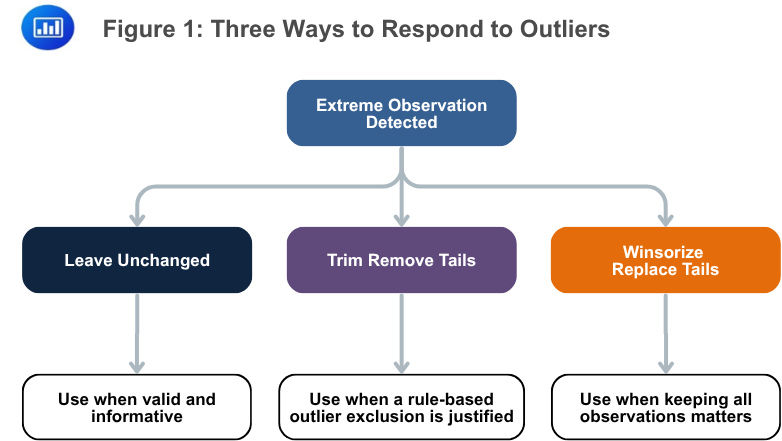
Figure 1 summarizes three practical responses. The analyst may leave outliers unchanged, remove them through trimming, or replace them through winsorizing. Leaving outliers unchanged preserves the full information in the original dataset. Trimming removes a stated percentage from the top and bottom tails before calculating the mean. Winsorizing keeps the number of observations unchanged but replaces extreme observations with specified percentile values.

A trimmed mean is calculated after removing a specified percentage of the lowest and highest observations. For example, a 10% trimmed mean removes 5% from the lower tail and 5% from the upper tail before the mean is calculated.

A winsorized mean is calculated after replacing extreme observations with less extreme percentile values. For example, a 90% winsorized mean may set observations below the 5th percentile equal to the 5th percentile value and observations above the 95th percentile equal to the 95th percentile value.

The practical distinction is important: trimming removes observations, while winsorizing replaces extreme values.

Example 2: Evaluating a Mean Distorted by Outliers

Suppose we want to compare the ordinary mean, a trimmed mean, and a winsorized mean for nine weekly returns on a commodity-linked exchange-traded fund. The sorted returns are:

$$
\begin{array}{c}
\textbf{Return} \\ \hline
-15.0\% \\ \hline
-3.0\% \\ \hline
-1.0\% \\ \hline
0.0\% \\ \hline
1.0\% \\ \hline
2.0\% \\ \hline
3.0\% \\ \hline
4.0\% \\ \hline
20.0\% \\
\end{array}
$$

The objective is to see how the two extreme observations affect the average.

Solution

Recall the mean formula:

$$
\bar{X} = \frac{1}{n} \sum_{i=1}^{n} X_i
$$

Where:

• \(\bar{X}\) is the sample mean weekly return
• \(n = 9\), the number of weekly returns
• \(X_i\) is the return in week \(i\)

The ordinary mean is:

$$ \begin{align*}
\bar{X} & = \frac{-15\% – 3\% – 1\% + 0\% + 1\% + 2\% + 3\% + 4\% + 20\%}{9} \\
\bar{X} & = 1.22\% \end{align*}
$$

For a simple trimmed calculation, remove the lowest and highest values. The remaining seven returns are -3.0%, -1.0%, 0.0%, 1.0%, 2.0%, 3.0%, and 4.0%. The trimmed mean is:

$$
\bar{X}_{\text{trimmed}} = \frac{-3\% – 1\% + 0\% + 1\% + 2\% + 3\% + 4\%}{7} = 0.86\%
$$

For a simple winsorized calculation, replace -15.0% with -3.0% and 20.0% with 4.0%. The winsorized data keep nine observations:

$$
-3\%,\, -3\%,\, -1\%,\, 0\%,\, 1\%,\, 2\%,\, 3\%,\, 4\%,\, 4\% $$

The winsorized mean is:

$$
\bar{X}_{\text{winsorized}} = \frac{7\%}{9} = 0.78\%
$$

The ordinary mean is highest because the positive outlier is larger in magnitude than the negative outlier. Trimming and winsorizing reduce the influence of extreme observations and move the average closer to the center of the weekly return pattern.

Quantiles and Measures of Location

A quantile identifies the value at or below which a stated fraction of the data lies. Quantiles are measures of location because they describe where observations sit within an ordered dataset.

Common quantiles include quartiles, quintiles, deciles, and percentiles.

$$ \textbf{Table 2: Common Quantiles}\\
\begin{array}{l|c|c}
\textbf{Quantile Type} & \textbf{Number of Groups} & \textbf{Typical Interpretation} \\ \hline
\text{Quartile} & 4 & \text{Divides data into four equal groups} \\ \hline
\text{Quintile} & 5 & \text{Divides data into five equal groups} \\ \hline
\text{Decile} & 10 & \text{Divides data into ten equal groups} \\ \hline
\text{Percentile} & 100 & \text{Shows relative standing on a 0-to-100 scale} \\
\end{array}
$$

Table 2 helps clarify language that often appears in manager research. In a performance-ranking context, a first-quartile manager may mean one of the best-performing managers. In a mathematical percentile context, a lower percentile may indicate a lower observed value. Candidates must read the context carefully.

The interquartile range measures the spread of the middle 50% of observations:

$$
IQR = Q_3 – Q_1
$$

Where:

• \(IQR\) is the interquartile range
• \(Q_3\) is the third quartile, or 75th percentile
• \(Q_1\) is the first quartile, or 25th percentile

The IQR is less sensitive to outliers than the full range because it ignores the most extreme lower and upper observations.

Figure 2: Box-and-Whisker Plot and the Interquartile Range

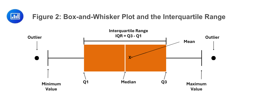
Figure 2 illustrates how a box-and-whisker plot summarizes location and dispersion. The box spans the interquartile range, from Q1 to Q3. The median lies inside the box. The whiskers extend to non-outlier values, while observations far beyond the whiskers can be flagged as potential outliers. The box, therefore, provides a compact view of the middle of the distribution and the potential extremes.

Example 3: Calculating the Interquartile Range

Suppose we want to describe the location and spread of annual excess returns for an equity factor strategy. The ordered returns are:

$$
\begin{array}{c}
\textbf{Ordered Return} \\ \hline
-8.0\% \\ \hline
-3.0\% \\ \hline
1.0\% \\ \hline
4.0\% \\ \hline
6.0\% \\ \hline
9.0\% \\ \hline
15.0\% \\
\end{array}
$$

Assume the first quartile is -3.0% and the third quartile is 9.0%. The objective is to calculate and interpret the interquartile range.

Solution

We know that:

$$
IQR = Q_3 – Q_1
$$

Where:

• \(Q_3 = 9.0\%\), the third quartile
• \(Q_1 = -3.0\%\), the first quartile
• \(IQR\) is the spread of the middle 50% of returns

Substituting the values:

$$
IQR = 9.0\% – (-3.0\%) = 12.0\%
$$

The middle 50% of annual excess returns spans 12.0 percentage points. The lowest and highest returns, -8.0% and 15.0%, do not directly determine the IQR, which makes it less sensitive to extremes than the range.

Dispersion and Risk

A measure of dispersion describes how spread out the observations are around a central value. In asset return analysis, dispersion is closely related to risk because it captures uncertainty around the expected or average outcome.

The simplest dispersion measure is the range:

$$
\text{Range} = X_{\text{max}} – X_{\text{min}}
$$

Where:

• \(\text{Range}\) is the distance between the highest and lowest values
• \(X_{\text{max}}\) is the maximum value in the dataset
• \(X_{\text{min}}\) is the minimum value in the dataset

The range is easy to calculate, but it uses only two observations. A dataset with one extreme outlier can have a very large range even if most observations are tightly clustered.

The mean absolute deviation is the average absolute distance between each observation and the sample mean:

$$
MAD = \frac{1}{n} \sum_{i=1}^{n} \left| X_i – \bar{X} \right|
$$

Where:

• \(MAD\) is the mean absolute deviation
• \(n\) is the number of observations
• \(X_i\) is observation \(i\)
• \(\bar{X}\) is the sample mean
• \(\left| X_i – \bar{X} \right|\) is the absolute deviation of observation \(i\) from the sample mean

The median absolute deviation is the median of the absolute deviations from the dataset median:
$$
\text{Median absolute deviation} = \text{Median}\left( \left| X_i – \text{Median}(X) \right| \right)
$$

Where:

• \(\text{Median absolute deviation}\) is the median of the absolute deviations from the dataset median
• \(X_i\) is observation \(i\)
• \(\text{Median}(X)\) is the median of the dataset
• \(\left| X_i – \text{Median}(X) \right|\) is the absolute deviation from the median

Median absolute deviation is a robust measure because it uses the median rather than the mean and focuses on the middle absolute deviation.

Example 4: Calculating Range and Mean Absolute Deviation

Suppose we want to summarize the dispersion of five annual returns for a multi-asset fund. The returns are:

$$
\begin{array}{l|c}
\textbf{Year} & \textbf{Return} \\ \hline
1 & -6.0\% \\ \hline
2 & 2.0\% \\ \hline
3 & 5.0\% \\ \hline
4 & 7.0\% \\ \hline
5 & 12.0\% \\
\end{array}
$$

The objective is to calculate the range and mean absolute deviation.

Solution

We know that:

$$
\text{Range} = X_{\text{max}} – X_{\text{min}}
$$

Where:

• \(X_{\text{max}} = 12.0\%\), the highest annual return
• \(X_{\text{min}} = -6.0\%\), the lowest annual return
• \(\text{Range}\) is the full spread between the highest and lowest returns

Substitute the values:

$$
\text{Range} = 12.0\% – (-6.0\%) = 18.0\%
$$

Recall:

$$
MAD = \frac{1}{n} \sum_{i=1}^{n} \left| X_i – \bar{X} \right|
$$

Where:

• \(n = 5\), the number of annual returns
• \(X_i\) is the return in year \(i\)
• \(\bar{X}\) is the sample mean annual return
• \(MAD\) is the average absolute deviation from the sample mean

First calculate the mean:

$$
\bar{X} = \frac{-6\% + 2\% + 5\% + 7\% + 12\%}{5} = 4.0\%
$$

Then calculate absolute deviations from the mean:

$$
\begin{array}{l|c}
\textbf{Return} & \textbf{Absolute Deviation from 4.0%} \\ \hline
-6.0\% & 10.0\% \\ \hline
2.0\% & 2.0\% \\ \hline
5.0\% & 1.0\% \\ \hline
7.0\% & 3.0\% \\ \hline
12.0\% & 8.0\% \\
\end{array}
$$

The mean absolute deviation is:

$$
MAD = \frac{10\% + 2\% + 1\% + 3\% + 8\%}{5} = 4.8\%
$$

The fund’s range is 18.0%, while its MAD is 4.8%. The range captures the full distance between the extreme observations; the MAD describes the average absolute distance from the mean.

Variance and Standard Deviation

Variance and standard deviation are the most widely used measures of dispersion in finance. They are based on squared deviations from the mean.

The population variance is given by:

$$
\sigma^2 = \frac{1}{n} \sum_{i=1}^{n} (X_i – \mu)^2
$$

Where:

• \(\sigma^2\) is the population variance
• \(n\) is the number of observations in the population
• \(X_i\) is observation \(i\)
• \(\mu\) is the population mean
• \((X_i – \mu)^2\) is the squared deviation from the population mean

The population standard deviation is:

$$
\sigma = \sqrt{\frac{1}{n} \sum_{i=1}^{n} (X_i – \mu)^2}
$$

Where:

• \(\sigma\) is the population standard deviation
• \(\sigma^2\) is the population variance
• \(n\) is the number of observations in the population
• \(X_i\) is observation \(i\)
• \(\mu\) is the population mean

When working with a sample, the sample variance uses the sample mean and divides by \(n – 1\):

$$
s^2 = \frac{1}{n-1} \sum_{i=1}^{n} (X_i – \bar{X})^2
$$

Where:

• \(s^2\) is the sample variance
• \(n\) is the number of sample observations
• \(X_i\) is observation \(i\)
• \(\bar{X}\) is the sample mean
• \(n – 1\) is the degrees of freedom used for Bessel’s correction

The sample standard deviation is:

$$
s = \sqrt{\frac{1}{n-1} \sum_{i=1}^{n} (X_i – \bar{X})^2}
$$

Where:

• \(s\) is the sample standard deviation
• \(s^2\) is the sample variance
• \(n\) is the number of sample observations
• \(X_i\) is observation \(i\)
• \(\bar{X}\) is the sample mean

Dividing by \(n – 1\) is called Bessel’s correction. It makes the sample variance an unbiased estimator of the population variance. The correction matters most when the sample is small. As the sample size becomes large, the difference between dividing by \(n\) and dividing by \(n – 1\) becomes much smaller.

Standard deviation is easier to interpret than variance because it is expressed in the same units as the original data. If returns are expressed as percentages, the standard deviation is also expressed as a percentage. Variance is expressed in squared return units, which is less intuitive.

Example 5: Calculating Sample Variance and Sample Standard Deviation

Suppose we wish to calculate the sample variance and standard deviation of four quarterly returns for a listed real estate fund. The returns are:

$$
\begin{array}{l|c}
\textbf{Quarter} & \textbf{Return} \\ \hline
1 & -4.0\% \\ \hline
2 & 2.0\% \\ \hline
3 & 6.0\% \\ \hline
4 & 8.0\% \\
\end{array}
$$

The objective is to measure the dispersion of quarterly returns around the sample mean.

Solution

The sample variance formula is given by:

$$
s^2 = \frac{1}{n-1} \sum_{i=1}^{n} (X_i – \bar{X})^2
$$

Where:

• \(s^2\) is the sample variance of quarterly returns
• \(n = 4\), the number of quarterly returns
• \(X_i\) is the return in quarter \(i\)
• \(\bar{X}\) is the sample mean quarterly return
• \(n – 1 = 3\), the degrees of freedom

First, calculate the sample mean:

$$
\bar{X} = \frac{-4\% + 2\% + 6\% + 8\%}{4} = 3.0\%
$$

Now calculate squared deviations:

$$
\begin{array}{l|c|c}
\textbf{Return} & \textbf{Deviation from Mean} & \textbf{Squared Deviation} \\ \hline
-4.0\% & -7.0\% & 0.0049 \\ \hline
2.0\% & -1.0\% & 0.0001 \\ \hline
6.0\% & 3.0\% & 0.0009 \\ \hline
8.0\% & 5.0\% & 0.0025 \\ \hline
\textbf{Total} & & 0.0084 \\
\end{array}
$$

The sample variance is:

$$
s^2 = \frac{0.0084}{3} = 0.0028
$$

Now quote the sample standard deviation formula:

$$
s = \sqrt{s^2}
$$

Where:

• \(s\) is the sample standard deviation of quarterly returns
• \(s^2 = 0.0028\), the sample variance

The sample standard deviation is:

$$
s = \sqrt{0.0028} = 5.29\%
$$

The quarterly sample standard deviation is 5.29%. The negative and positive deviations around the mean have been squared, so both contribute positively to the estimated dispersion.

Scaling Variance and Standard Deviation through Time

When returns are independently and identically distributed, variance scales approximately linearly with time:

$$
\sigma^2_T \approx T \sigma^2_{\text{period}}
$$

Where:

• \(\sigma^2_T\) is the variance over \(T\) periods
• \(T\) is the number of periods
• \(\sigma^2_{\text{period}}\) is the variance for one period

Standard deviation scales with the square root of time:

$$
\sigma_T \approx \sqrt{T} \sigma_{\text{period}}
$$

Where:

• \(\sigma_T\) is the standard deviation over \(T\) periods
• \(T\) is the number of periods
• \(\sigma_{\text{period}}\) is the standard deviation for one period

This relationship is often called the root-of-time rule. It is widely used in finance, but it is an approximation. Real return series can violate the assumptions behind the rule because of serial correlation, changing volatility, fat tails, market stress, or changing economic regimes.

Example 6: Scaling Daily Volatility to Monthly Volatility

Suppose we wish to estimate monthly volatility for a currency strategy using its daily standard deviation. The daily standard deviation is 0.75%, and the analyst assumes 21 trading days in a month.

Solution

We know that:

$$
\sigma_T \approx \sqrt{T} \sigma_{\text{period}}
$$

Where:

• \(\sigma_T\) is the estimated monthly standard deviation
• \(T = 21\), the assumed number of trading days in one month
• \(\sigma_{\text{period}} = 0.75\%\), the daily standard deviation

Substituting the values:

$$
\sigma_T \approx \sqrt{21}(0.75\%) = 3.44\%
$$

The estimated monthly standard deviation is 3.44%. The estimate assumes that daily returns are independent and that daily volatility remains stable across the month. If volatility is clustered or market conditions change sharply, realized monthly volatility may differ from the scaled estimate.

Interpretation and Evaluation

Several practical principles follow:

• The mean uses all observations but can be pulled by outliers
• The median is more robust because it depends on position rather than magnitude
• The mode identifies clustering and may be more useful as a modal interval for continuous returns
• Trimming removes extreme observations; winsorizing replaces extreme observations
• Quantiles describe location within an ordered dataset
• The interquartile range measures the spread of the middle 50% of observations
• The range is simple but depends only on two observations
• Mean absolute deviation uses all observations but is less common in modeling than variance and standard deviation
• Median absolute deviation is robust to outliers
• Sample variance uses \(n – 1\) because the sample mean is estimated from the same data
• Standard deviation is often interpreted as volatility because it is in the same unit as returns
• The root of time rule is useful but should be treated as an approximation

Question

A risk analyst observes the following five annual returns for a multi-strategy fund:

$$
\begin{array}{l|c}
\textbf{Year} & \textbf{Return} \\ \hline
1 & -10.0\% \\ \hline
2 & 2.0\% \\ \hline
3 & 4.0\% \\ \hline
4 & 6.0\% \\ \hline
5 & 8.0\% \\
\end{array}
$$

The fund’s sample standard deviation of annual returns is closest to:

1. 6.32%
2. 7.07%
3. 7.91%

The correct answer is B.

Recall that the sample variance formula is given by:

$$
s^2 = \frac{1}{n-1} \sum_{i=1}^{n} (X_i – \bar{X})^2
$$

Where:

• \(s^2\) is the sample variance of annual returns
• \(n = 5\), the number of annual returns
• \(X_i\) is the return in year \(i\)
• \(\bar{X}\) is the sample mean annual return
• \(n – 1 = 4\), the degrees of freedom

First, calculate the mean:

$$
\bar{X} = \frac{-10\% + 2\% + 4\% + 6\% + 8\%}{5} = 2.0\%
$$

The squared deviations are:

$$
\begin{array}{c|c|c}
\textbf{Return} & \textbf{Deviation from Mean} & \textbf{Squared Deviation} \\ \hline
-10.0\% & -12.0\% & 0.0144 \\ \hline
2.0\% & 0.0\% & 0.0000 \\ \hline
4.0\% & 2.0\% & 0.0004 \\ \hline
6.0\% & 4.0\% & 0.0016 \\ \hline
8.0\% & 6.0\% & 0.0036 \\ \hline
\textbf{Total} & & 0.0200 \\
\end{array}
$$

The sample variance is:

$$
s^2 = \frac{0.0200}{4} = 0.0050
$$

Now use the sample standard deviation formula:

$$
s = \sqrt{s^2}
$$

Where:

• \(s\) is the sample standard deviation of annual returns
• \(s^2 = 0.0050\), the sample variance

The sample standard deviation is:

$$
s = \sqrt{0.0050} = 7.07\%
$$

The fund’s sample standard deviation is approximately 7.07%.

A is incorrect because it is based on the population denominator, \(n = 5\), rather than the sample denominator, \(n – 1 = 4\)

C is incorrect because it overstates dispersion by using an incorrect sum of squared deviations