Cash Flow Additivity and No-Arbitrage Pricing: Forward Rates, FX Forwards, and Options

Cashflow Additivity Principle

According to the cashflow additivity principle, the present value of any sum of any future cashflows is equivalent to the sum of the present values of the associated cashflows. The cash flow additivity principle ensures that the no-arbitrage principle is adhered to in financial markets.

This principle has different applications in time value of money problems. Besides, this principle can be applied to different economic scenarios.

Application of Cashflow Additivity

Forward Exchange Rates and the No-Arbitrage Principle

The principle of cash flow additivity can be applied to scenarios involving different currencies by converting all cash flows to a common currency using the appropriate exchange rates. Doing so allows us to compare and combine cash flows from different currencies and make investment decisions based on their combined value.

For example, suppose we have two investment opportunities, one in US dollars and one in Euros. We can convert the expected cash flows from the Euros investment into US dollars using the appropriate exchange rates. Then, we can compare the combined value of the two investments and decide based on their relative values.

Dealing with different currencies assumes continuous compounding. Recall that the present value of a continuous compounding is given by:

$$ PV_0=FV_t e^{-t\times r} $$

Example: Applying the Cash Flow Additivity Principle

Consider an investor with USD 2,000 who wants to invest it for three months. The investor can choose between two options: investing in the US government debt or German government debt. The three-month US dollar risk-free interest rate is 3%, and that of the German Euro is 6%.

Option 1: Investing in US Government Debt

The investor can invest his USD 2,000 in a three-month US Treasury bill. This means that he lends the government USD 2,000, and it promises to pay him back with interest in three months. The interest is 3%, so after three months, he will receive:

Recall that,

$$ FV_t=2,000 \times e^{0.03 \times \frac {3}{12}}=\text{USD } 2,015 $$

Option 2: Investing in German Government Debt

The investor chooses to invest in German government debt. To do this, the investor must convert his USD 2,000 into Euros at the current exchange rate of EUR/USD = 0.9200 (1 USD = 0.9200 EUR). This means that the investor will receive \((2,000 \times 0.92)=\text{EUR } 1840\). He can then lend this money to the German government by investing in a three-month German Treasury bill. As such, after three months, the investor will receive:

$$ \begin{align*}
FV & =\text{EUR } 1840 \times e^{0.06 \times \frac {3}{12}} \\
& =\text{EUR } 1,867.81 \end{align*} $$

Assuming the investor wants his money in US dollars, we need to convert EUR1867.81 back to USD at the forward exchange rate of EUR/USD = 0.9270. This means that the investor will receive:

$$\frac {1,867.81}{0.9270}=\$2,014.9 \approx 2,015$$

Both options give you the same amount of money after three months: USD 2,015. The difference is that one option involves investing in US dollars, and the other involves converting your money into Euros and back into US dollars.

The forward exchange rate for EUR/USD at 0.9270 is important because it determines how much you, the investor, will receive when converting your Euros back into US dollars. If this rate differs from 0.9270 (above or below), there would be an arbitrage opportunity in converting Euros to dollars.

More on foreign exchange rates will be discussed later in the curriculum.

Implied Forward Rates and Cash Flow Additivity

Consider two zero-coupon bonds. Bond A has a maturity of two years and a yield of 2% per annum, while Bond B has a maturity of four years and a yield of 3%. An investor, who doesn’t seek to take advantage of price differences and is risk-neutral, has $1,000 to invest. The investor has two investment options that earn the same return.

Option 1: The investor can put their money into bond B now, which has an annual yield of 3% and pays out at the end of 4 years. The Future Value (FV) of this investment in four years, using the formula for compound interest, is:

$$ FV_4=PV_0 (1+r_4)^4=1000(1.03)^4=1,125.51 $$

Option 2: Alternatively, the investor can initially invest in bond A and, after two years, reinvest the proceeds at a forward rate \(F_{2,4}\), which represents a two-year forward rate starting in year two.

By the principle of cash flow additivity, a risk-neutral investor will be indifferent between Options 1 and 2. This is because the Future Values of both investments at the end of four years should be the same:

$$ FV_4=PV_0 (1+r_4)^4=PV_0 (1+r_2)^2(1+F_{2,4})^2 $$

In this scenario, this simplifies to:

$$ 1,125.51=1,000(1.02)^2 (1+F_{2,4})^2 $$

Solving this equation for the forward rate gives:

$$ \Rightarrow F_{2,4}=\left[\frac {1,125.51}{1,000(1.02)^2}\right]^{\frac{1}{2}}-1=4.01\% $$

Therefore, to prevent arbitrage opportunities, the forward rate \(F_{2,4}\) should be set to 4.01%. This ensures there is no risk-free profit potential, maintaining market efficiency.

Cashflow Additivity and Option Pricing

Cash flow additivity can be used to determine the fair price of an option contract. An option contract gives the buyer the right, but not the obligation, to buy (call) or sell (put) an underlying asset at a specified price within a certain period.

Cash flow additivity allows investors to compare different strategies and determine a no-arbitrage price for a financial instrument.

Example: Illustrating Cashflow Additivity in a Call Option

Consider a stock that costs $100 now. Assume its price might increase by 30% to $130 or decrease by 15% to $85 over the next year.

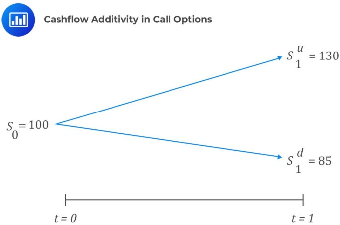
Let’s say an investor wants to sell a call on the stock that gives the buyer the right, but not the obligation, to purchase the asset for $120. The cash flow additivity principle can be used to determine the contract’s no-arbitrage price.

If the stock price goes up, the contract is worth \(c_1^u=10\). That’s because the buyer can use the contract to buy the asset for $120 and then sell it for $130, making a profit of $10. But if the price goes down, the contract is worth nothing. The buyer wouldn’t want to use the contract to buy the asset for $120 when they could just buy it for $85 without the contract.

The underlying argument here is that the value of the option is that each movement of the stock option may be used to construct a risk-free portfolio (the value of the portfolio is the same in both scenarios).

Denote the initial value of the call option by \(c_0\), which we wish to determine using cash flow additivity and no-arbitrage pricing. Also, denote the value of the portfolio at \(t=0\) by \(V_0\), when the stock price increases by \(V_1^u\) and when the stock price decreases by \(V_1^d\)

Assume that at \(t=0\) the investor creates a risk-free portfolio by selling a call option at \(c_0\) and buying 0.22 units of underlying assets. Then, the value of the portfolio at inception is:

$$ V_0=0.22 \times 100-c_0 $$

This portfolio is called a replicating portfolio because it is designed to create a matching future cash flow stream to that of a risk-free asset. The value 0.22 is the hedge ratio – the proportion of a position’s value that is hedged. In other words, it is the quantity of exposure that is sheltered against price.
Similarly, in each scenario of stock price decrease and increase:

$$ \begin{align*} V_1^u & =0.22 \times 130-10=18.89 \\
V_1^d & =0.22 \times 85-0=18.89 \end{align*} $$

Intuitively, the value-replicating portfolio equals 18.89, whether stock prices rise or decline. As such, the replicating portfolio is risk-free and can be discounted as a risk-free asset. Assuming that risk-free rate is r = 2.5%, then:

$$ \begin{align*}
V_0 & =V_1^u (1+r)^{-1}=V_1^d (1+r)^{-1} \\
& =18.89(1.025)^{-1}=18.43 \end{align*} $$

At this point, we can calculate the value of \(c_0\) rearranging the initial portfolio value equation:

$$ \begin{align*} V_0 & =0.22 \times 100-c_0 \\
\Rightarrow 18.43 & =0.22 \times 100-c_0 \\
\therefore c_0 & =3.57 \end{align*} $$

As such, the fair price of the call option is $3.57, which the seller expects to receive from the buyer.

Question

Mike Cardillo, CFA, is an American analyst evaluating the pricing of a one-year foreign exchange forward contract as part of a treasury hedging decision. The current spot exchange rate is quoted as USD/EUR 1.1200 (1 EUR = 1.1200 USD). One-year risk-free interest rates, expressed with continuous compounding, are 4.10% in the United States and 3.85% in the euro zone. The one-year USD/EUR forward exchange rate that ensures no-arbitrage opportunity is closest to:

1. USD/EUR 1.1171
2. USD/EUR 1.1200
3. USD/EUR 1.1228

Solution

The correct answer is C.

Using the cash flows additivity principle, we wish to compute the forward exchange rate that minimizes arbitrage opportunities.

In one year, an investment of USD 1 in the American risk-free rate amounts to:

$$1\times e^{0.0385}=1.04185$$

Now, if we first convert the 1 USD into euros and invest in the Euro risk-free rate, we have:

$$\frac{1}{1.1200} e^{0.0385}= EUR \ 0.92790$$

In order to convert EUR 0.92790 to USD 1.04185 (Adhering to the cash flow additivity principle), we need a forward rate of:

$$\frac{ USD\ 1.04185}{ EUR 0.92790}=USD/EUR \ 1.1228$$