Present Value of Bonds and Stocks: Discounting Expected Future Cash Flows

Introduction to Time Value of Money

The time value of money (TVM) is a fundamental financial concept. It emphasizes that a sum of money is worth more in the present than in the future. There are three key reasons supporting this principle:

• The concept of opportunity cost suggests that money available today can be invested and generate interest, increasing its value over time. By delaying the use of money, one forgoes potential investment opportunities and the growth they offer.
• Inflation poses a threat to the purchasing power of money in the future. Due to inflation, the same amount of money may buy fewer goods or services in the future compared to its present value. Consequently, having money now is advantageous, as its purchasing power diminishes over time.
• There is an element of uncertainty regarding future cash flows. Unexpected events or circumstances may prevent the receipt of money as planned, rendering it less reliable. Until the money is obtained, there is a level of uncertainty attached to its availability and utility.

The difference between the cash flows received today and those received in the future is computed using the required rate of return, or discount rate, usually denoted \( r \). The discount rate varies depending on the type of instrument, the timing, and the riskiness of the anticipated cash flows.

So in general, the key components of the time value of money include:

• Required rate of return, or Discount rate: The rate of discounting or compounding that you apply to an amount of money to calculate its present or future value.
• Time periods: The whole number of time periods over which a sum’s present or future value is calculated. These periods can be annually, semi-annually, quarterly, monthly, weekly, etc.
• Present value (PV): The amount of money you have today (or at time \( T = 0 \)) is referred to as the present value.
• Future value (FV): The accumulated amount of money you get after investing the original sum at a specific interest rate and for a given time period, say, two years.

Fundamental Formulas in Time Value of Money Calculations

Let,

\(FV_t\) = Future value at time \(t\).

\(PV_0\) = Present value.

\(r\) = Stated discount rate per period.

\(t\) = Number of compounding periods.

Then the future value \((FV)\) of an investment is given by:

$$ FV_t=PV(1+r)^t $$

If \(t\) is large such that \(N \rightarrow \infty\) the initial cashflow is compounded continuously:

$$ FV_t=PVe^{r\times t} $$

To find the present value of the investment, we rewrite the above formula so that:

$$ PV_0=FV(1+r)^{-t} $$

And for the continuous compounding, we have,

$$ PV_0=FV_t e^{-r\times t} $$

Example: Calculating the Present Value of continuously Compounded Cashflows

A fund continuously accumulates to $4,000 over ten years at a 10% annual interest rate. The present value of this fund is closest to:

Solution

From the question, \(FV_{10}\)=4,000, \(r\)=10%, \(t\)=10

So,

$$ PV_0=FV_{10} e^{-r\times t}=\$4,000 \times e^{-0.1\times 10}=\$1,471.5178 $$

Frequency of Compounding

When the frequency of compounding is more than once per year (quarterly, monthly, etc.), the formulas are analogously defined as:

$$ FV_t=PV_0 \left(1+\frac {r}{m} \right)^{m\times t} $$

Where:

\(FV_t\) = Future value at time \(t\).

\(PV_0\) = Present value.

\(m\) = number of compounding periods per year.

\(t\) = Investment duration in years.

\(m\times t\) = total number of compounding periods over the investment duration

\(r\) = annual nominal interest rate.

Intuitively, the formula for the \(PV\) is given by:

$$ PV_0=FV_t \left(1+ \frac {r}{m} \right)^{-m\times t} $$

From the above discussion, we can generally annualize a periodic interest rate by using the following equivalence equation:

$$\left(1+r_{\text{annual}}\right)= \left(1+\frac {r}{m} \right)^{m}$$

Making \( r_{\text{annual}}\) we get:

$$ r_{\text{annual}}=\left(1+\frac {r}{m} \right)^{m}-1$$

Where,

\(r_{\text{annual}}\) = annualized nominal interest rate

\(\frac {r}{m} \) = periodic interest rate

\(m\times t\) = total number of compounding periods over the investment duration per year

As such, assume a security earned a 5% return over the last 60 days. The annualized return is given by:

$$\begin{align} r_{\text{annual}} &= \left(1+\frac{r}{m}\right)^{m}-1 \\ &= \left(1+0.05\right)^{\frac{365}{60}}-1 \\ &= 34.56\% \end{align}$$

What if the security earned 1.5% over 2 weeks? Then the annualized return is

$$\begin{align} r_{\text{annual}} &= \left(1+\frac{r}{m}\right)^{m}-1 \\ &= \left(1+0.015\right)^{\frac{52}{2}}-1 \\ &= 47.27\% \end{align}$$

Annualizing returns provides a better way to compare returns across different investment time horizons.

Calculation using a Financial Calculator

For calculating \(FV_t\) and \(PV_0\) using the \(\text{BA II Plus}^{\text{TM}}\) Financial Calculator, use the following keys:

\(N\) = Number of compounding periods.

\(I/Y\) = Rate per period.

\(PV\) = Present value.

\(FV\) = Future value.

\(PMT\) = Payment per period.

\(CPT\) = Compute.

It is important to note that the sign of \(PV\) and \(FV\) will be opposite. For example, if \(PV\) is negative, then \(FV\) will be positive. Generally, an inflow is entered with a positive sign, while an outflow is entered as a negative sign in the calculator.

Time Value of Money in Fixed-income Instruments

Fixed-income instruments are debt securities where an issuer borrows money from an investor (lender) in exchange for a promised future payment. Examples of fixed-income instruments are bonds, loans, and notes.

The market discount rate for fixed-income instruments, also known as yield-to-maturity (YTM), is the interest rate investors require to invest in a specific instrument.

Cash Flow Patterns Associated with Fixed-Income Instruments

Cash flows from fixed-income instruments follow three general patterns: discount or no intermediate cash flows, periodic interest payments, and level payments or amortizing loans.

Discount Cash Flow Patterns

For discount cashflow patterns, an investor pays an initial discounted price \((PV_0)\) for the instrument (such as a bond or a loan) and gets one payment \((FV_t)\) at the end of maturity. \((FV_t)\) covers both interest and principal repayment at maturity.

The investor’s return is the interest earned, that is, the difference between the initial price and the principal \((FV_t – PV_0)\).

Discount bonds are often called zero-coupon bonds because they do not pay periodic interest (coupons).

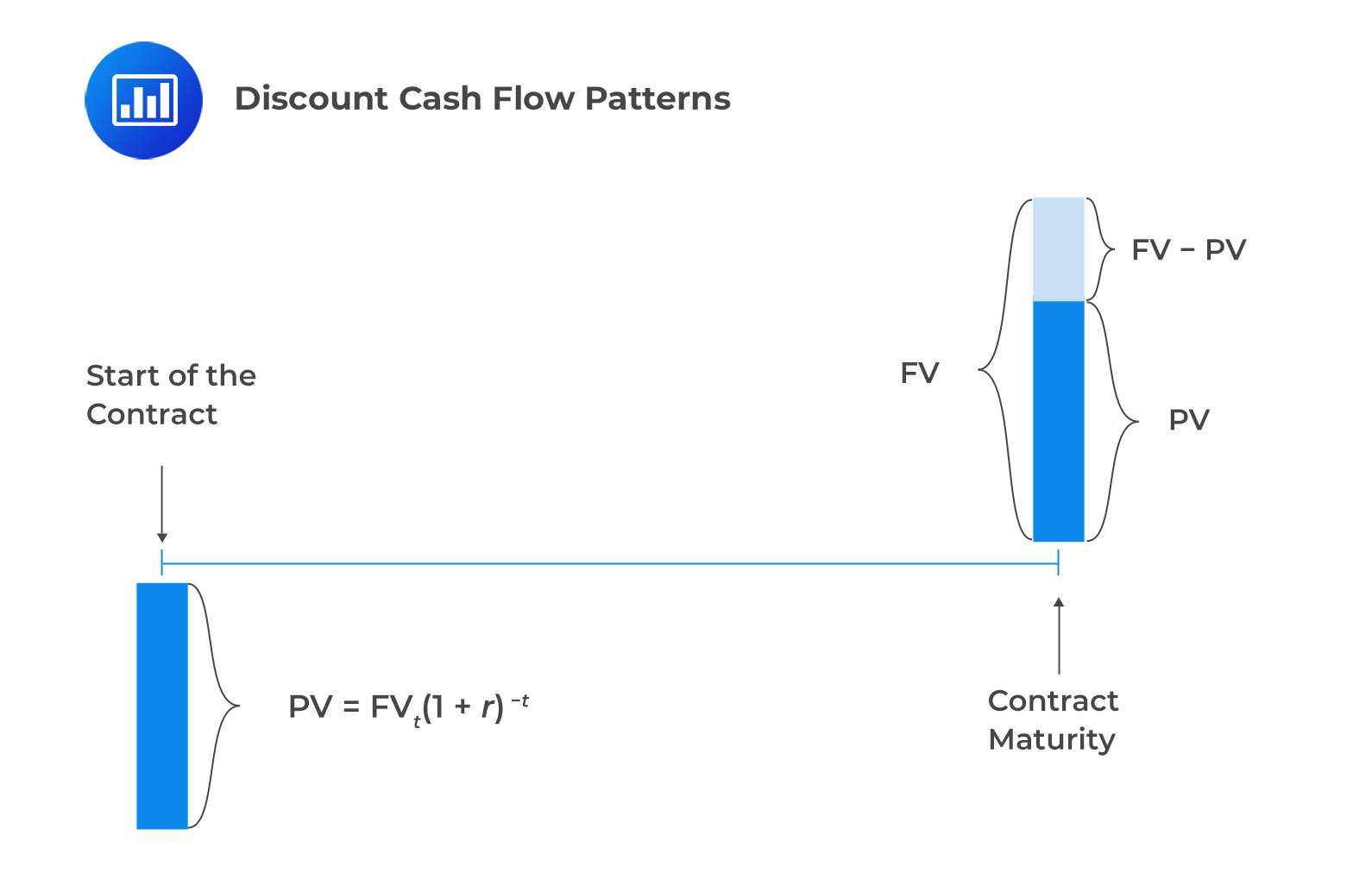
The price of a discount bond can be calculated using the formula for the present value \((PV)\) of a single cash flow, which is as follows:

$$ PV_{\text{Discount Bond}} =FV_t /(1+r)^{-t} $$

Where:

\(FV_t\) = Future value.

\(PV_0\) = Present value.

\(r\) = Stated discount rate per period.

\(t\) = Number of compounding periods.

Example: Calculating the Future Value of a Zero-Coupon Bond

Assume Chad invests $8,000 in a zero-coupon bond that yields 8% annually and matures in four years. The maturity value of this bond is closest to:

Solution

Recall that:

$$ FV_t= PV_{\text{Discount Bond}} (1+r)^t $$

In this case, we have \( PV_{\text{Discount Bond}} \)=8,000, \(r\)=8%, \(t\)=4 so that:

$$ FV=8,000(1+8\%)^4=10,883.91 $$

Using the \(\text{BA II Plus}^{\text{TM}}\) Financial Calculator

$$ \begin{array}{l|c|c}
\textbf{Steps} & \textbf{Explanation} & \textbf{Display} \\ \hline
{[\text{2nd}] [\text{QUIT}] }& \text{Return to standard calc Mode} & 0 \\ \hline
{[\text{2nd}] [\text{CLR TVM}] } & \text{Clears TVM Worksheet} & 0 \\ \hline
4[N] & \text{Years/periods} & N = 4 \\ \hline
8[1/Y] & \text{Set interest rate} & I/Y = 8 \\ \hline
-8,000[PV] & \text{Set present value} & PV = -8,000 \\ \hline
0[PMT] & \text{Set payment} & PMT = 0 \\ \hline
[CPT][FV] & \text{Compute future value} & FV = 10,883.91
\end{array} $$

Note that zero-coupon bonds can be issued at negative interest rates. In this case, the bond’s price (PV) exceeds its face value (FV).

Example: Calculating the Price of a Discount Bond Issued at Negative Interest Rates

In January 2018, the Swiss government issued 15-year sovereign bonds at a negative yield of -0.08%. The present value (PV) of the bond per CHF100 of principal (FV) at the time of issuance is closest to:

Solution

Recall for a zero-coupon bond,

$$ \begin{align*}
PV_{\text{Discount Bond}} & =FV_t (1+r)^{-t} \\
& =100(1-0.0008)^{-15}=101.21
\end{align*} $$

Periodic Interest Pattern (Coupon Instrument)

In this arrangement, the investor pays an initial price \(PV_0\) for an instrument such as a bond or a loan and receives intermittent cash interest payments called coupon payments and are denoted by \(PMT_t\), and a principal payment, \(FV_T\), at maturity.

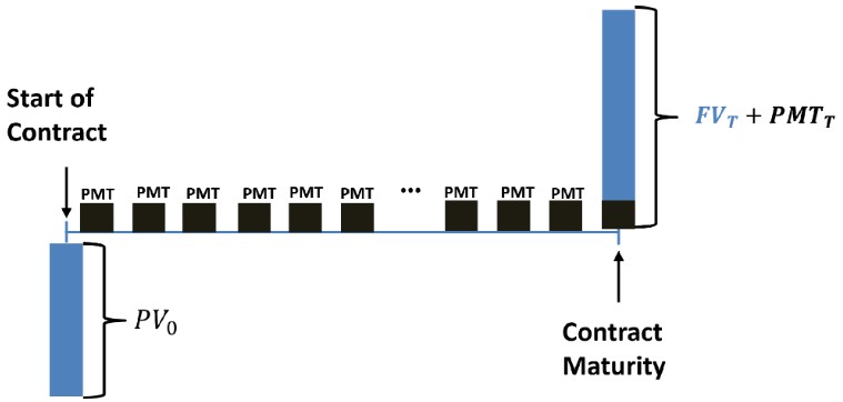
Coupon payments are made at predetermined intervals over the bond’s tenure, while the principal is paid at maturity. These types of bonds are generally called coupon bonds.

While keeping the time value of money in mind, the pricing of a coupon bond involves calculating its present value (\( PV_0 \)) using the market discount rate. The general formula for calculating the bond’s price is derived from the discounted cash flow model. It considers the coupon payments (PMTs) and the final principal payment (FV) at maturity. The bond’s price is determined by discounting each cash flow using the market discount rate (r).

The formula used to calculate the present value (PV) of a coupon bond is as follows:

$$
\begin{align}
PV_{\text{Coupon Bond}} &= \frac{PMT_1}{(1+r)^1} + \frac{PMT_2}{(1+r)^2} + \dots + \frac{PMT_t+FV_t}{(1+r)^t} \\
&= \sum_{t=1}^T \frac{PMT_t}{(1+r)^t} + \frac{FV_t}{(1+r)^t}
\end{align}
$$

Note that \( \sum_{t=1}^T \frac{PMT_t}{(1+r)^t} \) is a geometrical series which can be simplified as:

$$
\sum_{t=1}^T \frac{PMT_t}{(1+r)^t} = PMT \times \left[ \frac{1-(1+r)^{-T}}{r} \right] = \frac{PMT}{r} \times \left[ 1-\frac{1}{(1+r)^T} \right]
$$

As such, the closed-form formula for calculating a bond’s price is given by:

$$
PV_{\text{Coupon Bond}} = \frac{PMT}{r} \times \left[ 1-\frac{1}{(1+r)^T} \right] + \frac{FV_T}{(1+r)^T}
$$

Example 1: Pricing a Coupon Bond on an Annual Basis

Suppose we have a 5-year bond with a face value of $1,000 and an annual coupon rate of 5%. The market discount rate is 6%. The bond’s price is closest to:

Solution

$$ \text{PV(Coupon Bond)}=\frac {PMT}{(1+r)^1} + \frac {PMT}{(1+r)^2} +\dots +\frac {(PMT_N+FV_N)}{(1+r)^N} $$

In this case, we have \(PMT\)=5% of $1,000=$50, \(r\)=6%, \(N\)=5 years, \(FV\)=$1,000 so that:

$$ \begin{align*}
PV_{\text{Coupon Bond}} & =\frac {\$50}{(1+0.06)^1} +\frac {\$50}{(1+0.06)^2} + \frac {\$50}{(1+0.06)^3} + \frac {\$50}{(1+0.06)^4} \\ & + \frac {(\$50+\$1,000)}{(1+0.06)^5} \\ & =\$47.17+\$44.50+\$41.98+\$39.60+\$784.62=\$957.88 \\
\end{align*} $$

Therefore, the price of the bond would be \(\bf{\$957.88}\)

Using the closed-form formula,

$$ \begin{align}PV_{\text{Coupon Bond}} &=\frac{PMT}{r}\times \left[1-\frac{1}{(1+r)^T}\right]+\frac{FV_T}{(1+r)^T }\\ &=\frac{50}{0.06}\times \left[1-\frac{1}{1.06^5}\right]+\frac{1000}{(1.06)^5}=\$957.88\end{align}$$

You could use a BA II Plus Calculator to solve the above question (this method saves a lot of time):

$$ \begin{array}{l|c|c}
\textbf{Steps} & \textbf{Explanation} & \textbf{Display} \\ \hline
{[\text{2nd}] [\text{QUIT}]} & \text{Return to standard calc Mode} & 0 \\ \hline
{[\text{2nd}] [\text{CLR TVM}]} & \text{Clears TVM Worksheet} & 0 \\ \hline
{5[N]} & \text{Years/periods} & N = 5 \\ \hline
{6[1/Y]} & \text{Set interest rate} & I/Y = 6.00 \\ \hline
{50[PMT]} & \text{Set payment} & PMT = 50.00 \\ \hline
{1000[FV]} & \text{Set the face value} & FV=1000.00 \\ \hline
{[CPT][PV]} & \text{Compute the present value} & PV = -957.88
\end{array} $$

The yield to maturity, or the bond’s discount rate, is usually quoted on an annual basis. However, the majority of bonds issued by entities, such as public or private borrowers, pay dividends semi-annually or quarterly. In this case, the periodic payments can be annualized, or the annual payments can be adjusted accordingly for the payment frequency.

Example 2: Pricing a Coupon Bond with a Single Cash Flow on a Semi-Annual Basis

Assume an investor has a 2-year bond with a face value of $1000 and an annual coupon rate of 6%, paid semi-annually. The market discount rate is 5%. The price of the bond is closest to:

Solution

Using the closed-form formula,

$$ \begin{align}PV_{\text{Coupon Bond}} &=\frac{PMT}{r}\times \left[1-\frac{1}{(1+r)^T}\right]+\frac{FV_T}{(1+r)^t }\\ &=\frac{30}{0.025}\times \left[1-\frac{1}{1.025^4}\right]+\frac{1000}{(1.025)^4}=\bf{\$1,018.81}\end{align}$$

Where:

\(PMT\) = Coupon payments \(\left($1,000 \times \frac {6\%}{2} \right)=\$30\) in this case.
\(FV_T\) = Future value ($1,000 in this case).
\(r\) = Market discount rate (YTM), \(\left(\frac {(5\%)}{2}=2.5\%\right)\) per period in this case.
\(T\) = number of periods (4 periods in this case).
Therefore, the bond’s price is \(\bf{\$1,018.81}\)

You can easily use the BA II Plus calculator (or any other allowed financial calculator) to solve the above question.

$$ \begin{array}{l|c|c}
\textbf{Steps} & \textbf{Explanation} & \textbf{Display} \\ \hline
{[\text{2nd}] [\text{QUIT}]} & \text{Return to standard calc Mode} & 0 \\ \hline
{[\text{2nd}] [\text{CLR TVM}]} & \text{Clears TVM Worksheet} & 0 \\ \hline
{4[N]} & \text{Years/periods} & N = 4 \\ \hline
{2.5[1/Y]} & \text{Set interest rate} & I/Y = 2.50 \\ \hline
{30[PMT]} & \text{Set payment} & PMT = 30.00 \\ \hline
{1000[FV]} & \text{Set the face value} & FV=1000.00 \\ \hline
{[CPT][PV]} & \text{Compute the present value} & PV = -1,018.81
\end{array} $$

Bonds with Variable Coupon Payments

Bonds with variable coupon bonds are usually denoted as floating-rate bonds. These bonds typically have coupon payments at periodic intervals to accommodate market conditions reflected in the underlying index.

Valuing a floating-rate bond necessitates the use of a pricing model. For a fixed-rate bond (discussed above), the price is determined by the market discount rate r and the coupon payment per period, PMT. The formula to calculate this price is as follows:

\[PV = \frac{PMT}{(1 + r)} + \frac{PMT}{(1 + r)^{2}} + \ldots + \frac{PMT + FV}{(1 + r)^{T}}\]

Where:

\(PV =\) Present value, or the price of the bond

\(PMT\) = Coupon payment per period

\(r =\) The market discount rate

\(FV\) = The future value paid at maturity, or the par value of the bond

\(T=\) The number of evenly spaced periods to maturity

In the context of a floating rate bond, PMT is derived from the Market Reference Rate (MRR) and the quoted margin. \(r\) is influenced by the MRR and the margin. The price of a floating rate bond is calculated using the formula:

For an FRN, the price is calculated using the following formula:

\[PV = \frac{\frac{(MRR + QM) \times FV)\ }{m}}{\left( 1 + \frac{MRR + DM}{m} \right)} + \frac{\frac{(MRR + QM) \times FV)\ }{m}}{\left( 1 + \frac{MRR + DM}{m} \right)^{2}} + \ldots + \frac{\frac{(MRR + QM) \times FV)\ }{m} + FV}{\left( 1 + \frac{MRR + DM}{m} \right)^{N}}\]

Where:

• \(PV =\) Present value, or the price of the floating-rate note
• \(MRR\) = The market reference rate, stated as an annual percentage rate
• \(QM =\) The quoted margin, stated as an annual percentage rate
• \(FV\) = The future value paid at maturity, or the par value of the bond
• \(m =\) The periodicity of the floating-rate note, the number of payment periods per year
• \(DM =\) The discount margin \(=\) required margin stated as an annual percentage rate
• \(N =\) The number of evenly spaced periods to maturity

Example: Calculating the Price of a Floating-Rate Note

Suppose we are pricing a three-year, semi-annual FRN that pays MRR plus \(0.75\%\). Assume MRR is \(1.50\%\) and the yield spread required by investors is 50bps. Given:

• MRR = 0.0150
• QM = 0.0075
• FV = 100
• m = 2
• DM = 0.0050
• N = 6

Calculate the price of the floating rate instrument.

Solution

Determine the coupon payment for each period:

$$\begin{align} PMT &= \frac{MRR + QM}{m} \times FV \\ &= \frac{0.0150 + 0.0075}{2} \times 100 \\ &= \frac{0.0225}{2} \times 100 = 1.125 \end{align}$$

Calculate the present value of each cash flow: For \(t = 1\) to \(T\) :

\[PV_{t} = \frac{PMT}{\left( 1 + \frac{(MRR + DM)}{m} \right)^{t}}\]

E.g., for t=1

\[PV_{1} = \frac{1.125}{\left( 1 + \frac{0.0150 + 0.0050}{2} \right)^{1}} = \ 1.1139\]

Finally, the price of the floating rate bond is the sum of all present values plus the present value of the face value at maturity:

\[\text{Price} = \sum_{t = 1}^{T}PV_{t} + \frac{FV}{\left( 1 + \frac{MRR + DM}{m} \right)^{T}}\]

The price of the FRN has been calculated as: 100.724

Perpetual Bonds

Perpetual bonds are a rare type of coupon bond that do not have a stated maturity date. They are generally issued by firms seeking equity-like financing and usually include redemption provisions.

The formula present value of perpetual bonds is obtained as follows: As \(N \rightarrow \infty\), the formula for calculating PV of coupon changes as follows:

$$ \begin{align*} \text{PV}_{\text{Perpetual bond}} &= \lim_{T \rightarrow \infty} \left[ \frac{PMT}{(1+r)^1} +\frac{PMT}{(1+r)^2} +\dots +\frac{(PMT_T+FV_T)}{(1+r)^T} \right] \\ &= \frac{PMT}{r} \end{align*} $$

So, the present value of a perpetuity is given by:

$$ PV=\frac {PMT}{r} $$

Example: Perpetual Bond

A hypothetical company, XYZ Financial, issued $500 million in perpetual bonds with a 4.00% semi-annual coupon. Calculate the bond’s yield to maturity (YTM) if the market price was $98.50 (per $100).

Solution

Recall,

$$ PV_{\text{Perpetual bond}}=\frac{PMT}{r} $$

Hence,

$$r=\frac {PMT}{ PV_{\text{Perpetual bond}}} $$

To solve this problem, we first need to calculate the semi-annual coupon payment, which is,

$$
\text{PMT(semi-annual coupon payment)}=\frac {\$100 \times 4\%}{2} = \$2,PV=\$98.50 $$

Therefore,

$$ r=\frac {\$2}{\$98.50}=0.0203=2.03\% $$
The annualized yield-to-maturity is:
$$ r=0.0203 \times 2 \approx 4.06\% $$

Level Payments (Annuity Instruments) Patterns

An annuity is a finite series of cash flows, all with the same value. A fixed-income instrument with annuity payments provides a stream of periodic equal cash inflows over a finite period.

Level payments consist of interest and principal. Fixed income instruments with level payments include fully amortizing loans and mortgages.

There are two types of annuities: ordinary annuities and annuities due. An annuity due is a type of annuity where payments start immediately at the beginning of time, at time \(t = 0\). In other words, payments are made at the beginning of each period.

On the other hand, an ordinary annuity is one in which cash flows occur at the end of each period. Such payments are said to be made in arrears (beginning at time t = 1). We shall consider an ordinary annuity in this section.

Ordinary Annuity

Remember that in an ordinary annuity, the series of payments does not begin immediately. Instead, payments are made at the end of each period. It is further worth noting that the present value of an annuity is equal to the sum of the current value of each annuity payment:

$$\begin{align*} PV_0&=PMT(1+r)^{-1}+PMT(1+r)^{-2}+…+PMT(1+r)^{-t-1}+PMT(1+r)^{-t} \\& =PMT (1+r)^{-1}+(1+r)^{-2}+…+(1+r)^{-(T-1)}+(1+r)^{-t} \\& =\frac{PMT}{r}\times \left[ 1-\frac{1}{(1+r)^t}\right]\end{align*} $$

Where:

\(PMT\) = Periodic cash flow.

\(r\) = Market interest rate per.

\(PV_0\) = Present value/ Principal Amount of the loan or bond.

\(t\) = Number of payment periods.

The periodic annuity is calculated as follows:

$$ PMT=\frac {r\times PV_0}{(1-(1+r)^{-t} } $$

Consider a fully amortizing mortgage loan. In this case, the borrower receives the mortgage loan now and agrees to make periodic payments equal to the sum of interest and principal payments.

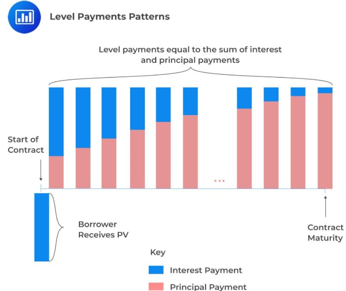
Note that the periodic mortgage payment is constant, but the proportion of the interest payment decreases while the principal payment increases.
The cash flow pattern of a fully amortizing mortgage resembles that of an ordinary annuity, with equal cash flows. As such, the periodic annuity (periodic payment) of a fully amortizing mortgage is given by:

$$ PMT=\frac {r\times PV_0}{(1-(1+r)^{-t} } $$

Where:

\(PMT\) = Periodic cash flow.

\(r\) = Market interest rate per period.

\(PV_0\) = Present value or principal amount of loan or bond.

\(t\) = Number of payment periods.

Example: Calculating the Periodic Payment of a Mortgage

Jake is looking to secure a fixed-rate 25-year mortgage to finance 75% of the value of an $800,000 residential property. If the annual interest rate on the mortgage is 4.5%, Jake’s monthly mortgage payment is close to:

Solution

Remember,

$$ PMT=\frac {r\times PV_0}{(1-(1+r)^{-t} } $$

Where:

\(A\) = Periodic cash flow.

\(r\) = Market interest rate per period.

\(PV_0\) = Present value/ Principal Amount of the loan or bond.

\(t\) = Number of payment periods.

In this case, we have:

• \(r = 0.375\% \left(=\frac {4.5\%}{12}\right)\)
• \(N=300 \text{ months} (=25 \text{ years} \times 12 \text{ months/year})\)
• \(PV=\$600,000 (=75\% \times \$800,000)\)

Plugging these values into the formula, we get:

$$ PMT=\frac {0.00375 \times \$600,000}{1-(1+0.00375)^{-300} }=\$3,334.995 \approx \$3,335 $$

Using a BA II Plus financial calculator (easier and less time-consuming):

$$ \begin{array}{l|c|c}
\textbf{Steps} & \textbf{Explanation} & \textbf{Display} \\ \hline
{[\text{2nd}] [\text{QUIT}]} & \text{Return to standard calc Mode} & 0 \\ \hline
{[\text{2nd}] [\text{CLR TVM}]} & \text{Clears TVM Worksheet} & 0 \\ \hline
{300[N]} & \text{Years/periods} & N = 300 \\ \hline
{0.375[1/Y]} & \text{Set interest rate} & I/Y = 0.375 \\ \hline
-600,000[PV] & {\text{Set the present value} } & PV = -600,000.00 \\
& {\text{of the mortgage}} & \\ \hline
{0[FV]} & \text{Set the face value} & FV=0.00 \\ \hline
{[CPT][PMT]} & \text{Compute the periodic payment} & PMT= 3,334.99
\end{array} $$

While considering the above formula, let us analyze the principal amortization and interest breakdown for the first and second months.

First month:

• The interest payment is calculated as: \(0.375\%\times 600,000)=\$2,250\)
• The principal amortization can be calculated as: PMT- Interest Payment
  
  $$3,334.99-2,250=1,084.99$$
• So, the remaining principal after the first month is:
  
  $$600,000-1,084.99=598,915.01$$

Second month

• The interest payment is calculated from the remaining principal after the first month has lapsed: \(0.375\%\times 598,915.01)=\$2,245.93\)
• Intuitively, the principal amortization for the second month is given as:
  
  $$3,334.99-2,245.93=1,089.06$$
• So, the remaining principal after the first month is:
  
  $$598,915.01-1,089.06=597,825.95$$

This process continues every month so that at maturity, the principal balance reduces to zero, and the final payment completes the loan repayment.

Time Value of Money in Equity Instruments

Equity investments, such as stocks, enable an investor to acquire a fractional share of ownership in the issuing company. This gives investors the right to receive a share of the company’s available cash flows as dividends.

In the context of equity instruments, the time value of money (TVM) is used to discount expected future cash flows to determine their present value. This allows investors to value the company shares.

The present value of expected future cash flows is calculated using a discount rate, r, which represents the expected rate of return on the investment.

Common Approaches for Valuing Equity Instruments

Valuing equity investments depends on dividend cash flows, which can take one of three forms: constant dividends, constant dividend growth rate, or changing dividend growth rate.

1. Valuing Equity Instruments based on Constant Dividend:The Constant Dividends model values stocks based on the assumption that dividends will remain constant over time. That is, the investor pays an initial price, \(PV_t\), for a preferred or common share and expects to receive a constant periodic dividend, \(Div_t\). The formula for the constant dividends model is as follows:$$ PV_t=\sum_{i=1}^\infty {\frac{Div_{t+1}}{(1+r)^i}} =\frac {Div_{t+1}}{r} $$Where:\(PV_t\) = Present value at time \(t\)
   

   \(Div_{t+1}\) =Expected dividend payment at the next payment period\(t+1\)

   
   

   \(r\) = Discount rate.

   
   

   Example: Valuing Equity Instruments based on Constant Dividend

   
   

   Assume we have a preferred stock with a $5 dividend payment next year. The discount rate is 8%. The present value of the stock is closest to:

   
   

   Solution

   
   

   Recall,

   
   

   $$ PV_t=\frac {Div_{t+1}}{r} $$

   
   

   In this case, \(Div_{t+1}\)=$5, \(r\)=8%, \(PV\)=?

   
   

   So,

   
   

   $$ PV=\frac {5}{0.08}=\$62.5 $$

   
   

   This means that the present value of the stock is $62.5.

2. Valuing Equity Instruments Based on Constant Dividend Growth Rate:The constant dividend growth model is a method used to estimate the value of a stock based on its future dividends. This model assumes that dividends will grow at a constant rate (g) forever. To derive the formula for this model, we start by considering that the present value of a stock is equal to the sum of its future dividends, discounted by the required rate of return \(r\). If dividends are assumed to grow at a constant rate, then each future dividend can be calculated by multiplying the previous dividend by \((1 + g)\).Let \(D_{t+1}\) represent the expected dividend in the next period. That is:$$Div_{t+1}=Div_t (1+g)$$The above formula can be applied for \(i\) period so that:
   

   $$Div_{t+i}=Div_i (1+g)$$

   
   

   Therefore, the present value of the stock can then be expressed as:

   
   

   $$ PV_0 =\sum_{i=1}^\infty \frac {Div_i (1+g)^i}{(1+r)^i}$$

   
   

   Which can be algebraically transformed into:

   
   

   $$ PV_0 = \frac {Div_0 (1+g)}{r-g}=\frac{Div_1}{r-g}$$

   
   

   With that in mind, we can now generalize the formula as:

   
   

   $$ PV_0 = \frac {Div_t (1+g)}{r-g}=\frac{Div_{t+1}}{r-g}, \text{for all}\ r-g>0$$

   
   

   Therefore, this is the formula for calculating the present value of a stock using the constant dividend growth rate. This model can help estimate a stock’s value when its future dividends are expected to grow steadily.

   
   

   Example: Valuing Equity Instruments based on Constant Dividend Growth Rate

   
   

   Suppose a stock currently pays an annual dividend of $2.00 per share. The required rate of return for this stock is 10%, and dividends are expected to grow at a constant rate of 5% per year indefinitely. Using the constant dividend growth model, the present value of this stock is closest to:

   
   

   Solution

   
   

   Recall that,

   
   

   $$ PV_0 = \frac {Div_t (1+g)}{r-g}=\frac{Div_{t+1}}{r-g}, \text{for all}\ r-g>0$$

   
   

   In this case, we know that \(D_t\)=$2.00, \(r\)=10%, \(g\)=5%

   
   

   So,

   
   

   $$ PV=\frac {2 \times 1.05}{r-g}=\frac {2.10}{0.10-0.05}=\$42 $$

   
   

   Therefore, the present value of the stock is $42

3. Valuing Equity Instruments with Changing Dividend Growth RatesValuing equity instruments with changing dividend growth rates requires a dynamic process. It begins with the investor buying a stock at an initial price and getting dividends under different growth rates. The unique aspect is that the dividend is expected to grow at a rate that evolves as the company matures, shifting from high growth to slower growth. This valuation doesn’t have a single formula because it relies on assumptions about future dividend growth. However, a common method is to use a multi-stage dividend discount model.The multi-stage dividend discount model assumes that dividends will grow at different rates during various stages of the company’s growth. To find the stock’s present value, you sum up the present values of dividends at each stage.The multi-stage dividend discount model builds on the constant dividend growth model discussed above. It accommodates a company’s transition from high initial growth to lower, more stable growth.
   

   Let’s say a company has a high short-term growth rate \(g_s\) followed by a perpetual lower growth rate \(g_l\). To find the present value (PV) of the stock at time \(t\) using this model, we compute it in two stages:

   
   
   
   
   1. First Part: The first part calculates the present value of dividends during the initial \(n\) periods of higher growth \((g_s)\). This is done by discounting the dividends for each period by the required rate of return r using the following formula:$$ PV_{\text{short-term dividend growth rate}}=\sum_{i=1}^n \frac {Div_t (1+g_s )^i}{(1+r)^i} $$Where:\(PV\) = Present value.\(n\) = Number of periods.\(D_t\) = Dividend at time (t).
      

      \(g_s\) = Initial higher dividend growth rate.

      
      

      \(r\) = Required rate of return.

   
   
   2. Second Part: The second part calculates the present value of dividends after the initial n periods, assuming constant growth at a lower long-term rate \((g_l)\). This can be simplified using the geometric series simplification, where \(E(S_t+n)\) represents the terminal value or stock value in n periods: $$ PV_{\text{long-term dividend growth rate}}=\frac { E(S_t+n)}{(1+r)^n} $$Where:\(E(S_t+n) = \frac {Div_{t+n+1}}{(r-g_l)}\)\(g_l\) = The lower, more stable dividend growth rate.
   
   
   
   

   As such, if we sum the first and second parts, we get the price of the stock:

   
   

   $$\begin{align}PV_0&=\sum_{i=1}^n \frac {Div_t (1+g_s )^i}{(1+r)^i}+\frac { E(S_t+n)}{(1+r)^n}\\ &=\sum_{i=1}^n \frac {Div_t (1+g_s )^i}{(1+r)^i}=\frac { \frac {Div_{t+n+1}}{(r-g_l)}}{(1+r)^n}\end{align}$$

   
   

   Example: Valuing Equity Instruments based on Changing Dividend Growth Rate

   
   

   A stock is currently paying an annual dividend of $2. The required rate of return is 10%. Dividends are expected to grow at 20% per year for the next three years, after which the growth rate will slow to 5% per year indefinitely.

   
   

   The present value (intrinsic value) of the stock is closest to:

   
   

   Solution

   
   

   First, we calculate the present value of the dividends during the high growth period:

   
   

   Recall that,

   
   

   $$ PV_t=\sum_{i=1}^n {\frac {Div_t (1+g_s )^i}{(1+r)^i}} $$

   
   

   In this case, \(Div_t\)=$2, \(g_s\)=0.20, \(r\)=0.10, \(n\)=3

   
   

   So,

   
   

   $$ \begin{align*}
   
   PV_{\text{Dividends}} & = \frac {2 \times (1+0.20)}{1+0.10)^1} + \frac {2 \times (1+0.20)^2}{1+0.10)^2} +\frac {2 \times (1+0.20)^3}{1+0.10)^3} \\
   
   & =2.182+2.380+2.596=7.158 \\
   
   & = \$7.158
   
   \end{align*} $$

   
   

   Next, we calculate the present value of the dividends during the slower growth period, assuming that dividends will grow at a constant rate of 5% thereafter:

   
   

   Recall that,

   
   

   $$ E(S_t+n)= \frac {Div_{t+n+1}}{(r-g_l ) } $$

   
   

   So,

   
   

   $$ E(S_t+3)=\frac { 2(1+0.20)^3 \times (1+0.05)}{ 0.10-0.05 }=\$72.576 $$

   
   

   Finally, we calculate the present value of this value of \(E(S_t+3)\) as:

   
   

   $$ =\frac {\$72.576 }{(1+0.10)^3} =\$54.50 $$

   
   

   The total present value of the stock is the sum of the above values.

   
   

   $$ \begin{align*}
   
   PV_0 & =\sum_{i=1}^n \frac {Div_t (1+g_s )^i}{(1+r)^i}+\frac { E(S_t+n)}{(1+r)^n}\\
   
   &=\$7.158+\$54.50 \\
   
   & =\$61.66
   
   \end{align*} $$

Question

Five years ago, Milton Inc. issued corporate bonds with a 15-year maturity. The bonds have a semi-annual coupon rate of 7.8% per annum, and the current yield to maturity is 8.5% per annum. The current price of Milton Inc’s bonds (per CAD100 of par value) is closest to:

1. 91.23
2. 95.35
3. 93.15

The correct answer is B.

Solution

Recall the formula for calculating the price of a bond:

$$ PV_{\text{Coupon Bond}} =\frac{PMT}{r}\times \left[1-\frac{1}{(1+r)^T}\right]+\frac{FV_T}{(1+r)^T }$$

First, let’s get the semi-annual equivalent rates:

• The semi-annual coupon rate is \(\frac{7.8\%}{2} = 3.9\%\).
• The semi-annual yield to maturity is \(\frac{8.5\%}{2} = 4.25\%\).

Next, we find the number of periods remaining until the bond matures:

Since the bonds were issued 5 years ago and have a 15-year maturity, \(10 (=15 – 5)\) years remain to maturity. Since interest is paid semi-annually, this equates to \(10\times 2 = 20\) periods.

So,

$$ PV_{\text{Coupon Bond}} =\frac{3.9}{0.0425}\times \left[1-\frac{1}{(1+0.0425)^{20}}\right]+\frac{100}{(1+0.0425)^{20} }=95.35 $$

You can plug the values above into the general formula, wasting valuable time. Therefore, using BA II plus a financial calculator,

$$ \begin{array}{l|c|c}
\textbf{Steps} & \textbf{Explanation} & \textbf{Display} \\ \hline
{[\text{2nd}] [\text{QUIT}]} & \text{Return to standard calc Mode} & 0 \\ \hline
{[\text{2nd}] [\text{CLR TVM}]} & \text{Clears TVM Worksheet} & 0 \\ \hline
{20[N]} & \text{Years/periods} & N = 20 \\ \hline
{4.25[1/Y]} & \text{Set interest rate} & I/Y = 4.25 \\ \hline
3.9[PMT] & {\text{Set the periodic} } & PMT = 3.90 \\
& {\text{coupon payment}} & \\ \hline
{100[FV]} & \text{Set the face} & FV= 100.00 \\
& \text{value of the bond} & \\ \hline
{[CPT][PV]} & \text{Compute the present value} & PV = -95.35
\end{array} $$