Key Statistical Distributions in Finance: Mean, Variance, Skewness, and Kurtosis

Why Distributions Matter in Investment Work

The first learning outcome introduced the basic machinery of random variables, probability functions, expected value, variance, and covariance. This one, on the other hand, moves from general probability tools to the specific statistical distributions most often used in finance. The practical question changes from, “How do we calculate a mean or variance?” to, “Which distribution describes this investment problem, and what do its moments tell us?”

A distribution is not chosen because it looks elegant on paper. It is chosen because it reflects the economic structure of the problem being modeled. A portfolio manager modeling monthly returns, a credit analyst modeling default counts, and a quant researcher modeling the number of profitable trading signals are not all dealing with the same kind of uncertainty. The distribution should match the type of outcome, the range of possible values, and the shape of the risk.

The principal moments summarize that shape. The mean gives the center of the distribution. The variance measures dispersion around that center. Skewness describes asymmetry, and excess kurtosis tells us whether the tails are heavier or lighter than those of a normal distribution. In finance, these moments matter because return distributions often have features that a simple mean cannot capture: downside asymmetry, rare but severe losses, clustered events, and heavy tails.

The Four Moments

Before discussing the individual distributions, it is useful to keep the four moments in view.

$$ \textbf{Table 1: The Four Principal Moments} \\
\begin{array}{l|c|c}
\textbf{Moment} & \textbf{What It Measures} & \textbf{Investment Interpretation} \\
\hline
\text{Mean} & \text{Center of the distribution} & {\text{Expected value, average count,} \\ \text{or central tendency} }\\
\hline
\text{Variance} & \text{Spread around the mean} & {\text{Volatility, uncertainty, or} \\ \text{dispersion of outcomes}} \\
\hline
\text{Skewness} & \text{Asymmetry of the distribution} & {\text{Whether extreme outcomes are} \\ \text{more likely on one side}} \\
\hline
\text{Excess kurtosis} & {\text{Tail heaviness relative to} \\ \text{the normal distribution}} & {\text{Whether extreme outcomes} \\ \text{are more frequent than} \\ \text{normality would imply}} \\
\end{array}
$$

Table 1 is a useful exam map. A question that asks for the mean is asking about the center. A question that asks for the variance is asking about spread. A question about skewness is asking about asymmetry. Finally, a question about excess kurtosis concerns tail behavior relative to the normal distribution.

Choosing the Distribution

A strong analyst does not memorize distributions as isolated formulas. They identify the investment problem and then choose the probability model that best fits its structure.

$$ \textbf{Table 2: Common Distributions and Typical Financial Uses} \\
\begin{array}{l|c|c|c}
\textbf{Distribution} & \textbf{Type} & \textbf{Typical Finance Use} & \textbf{Key Feature} \\
\hline
\text{Discrete uniform} & \text{Discrete} & \text{Equally likely discrete outcomes} & {\text{Every outcome has the} \\ \text{same probability}} \\
\hline
\text{Binomial} & \text{Discrete} & {\text{Number of successes in} \\ \text{fixed independent trials}} & {\text{Two possible outcomes} \\ \text{per trial}} \\
\hline
\text{Poisson} & \text{Discrete} & {\text{Rare event counts} \\ \text{over time or space}} & {\text{Mean equals variance} \\ \text{for a given interval}} \\
\hline
\text{Continuous uniform} & \text{Continuous} & {\text{Simulation inputs and} \\ \text{equally likely ranges}} & \text{Flat density over an interval} \\
\hline
\text{Normal} & \text{Continuous} & {\text{Returns, errors, and} \\ \text{statistical inference}} & {\text{Symmetric bell-shaped} \\ \text{distribution}} \\
\hline
\text{Log-normal} & \text{Continuous} & {\text{Asset prices and other} \\ \text{non-negative variables}} & {\text{Values are positive} \\ \text{and right-skewed}} \\
\hline
\text{Logistic} & \text{Continuous} & {\text{Logistic regression and} \\ \text{binary classification}} & {\text{Symmetric, heavier-tailed} \\ \text{than normal}} \\
\end{array}
$$

Discrete Uniform Distribution

A discrete uniform distribution applies when a finite number of possible outcomes are equally likely. A fair six-sided die is the classic classroom example, but the same idea can appear in finance when an analyst intentionally assigns equal probability to a small set of discrete scenarios. For example, a stress-testing team might begin with five equally weighted liquidity scenarios before replacing the equal weights with more refined probabilities.

For a discrete uniform distribution with integer outcomes from \(a\) to \(b\), the mean is:

$$
\begin{align}
\mu = \frac{a+b}{2}
\end{align}
$$

Where:

• \(\mu\) is the mean of the discrete uniform distribution
• \(a\) is the smallest possible value
• \(b\) is the largest possible value

The variance is:

$$
\begin{align}
\sigma^2 = \frac{(b-a+1)^2-1}{12}
\end{align}
$$

Where:

• \(\sigma^2\) is the variance of the discrete uniform distribution
• \(a\) is the smallest possible value
• \(b\) is the largest possible value
• \(b – a + 1\) is the number of equally likely integer outcomes

The distribution is symmetric when the outcomes are evenly spaced. Its skewness is therefore zero. The variance increases as the range between \(a\) and \(b\) widens.

Example 1: Discrete Uniform Scenario Scores

A risk committee assigns equal likelihood to five cybersecurity disruption scores for a digital bank: 1, 2, 3, 4, and 5, where 1 indicates a very small disruption and 5 indicates a severe disruption.  Find the mean and variance.

Solution

Start by quoting the formula:

$$
\begin{align}
\mu = \frac{a+b}{2}
\end{align}
$$

$$
\begin{align}
\sigma^2 = \frac{(b-a+1)^2-1}{12}
\end{align}
$$

The mean disruption score is:

$$
\begin{align}
\mu = \frac{1+5}{2} = 3
\end{align}
$$

The variance is:

$$
\begin{align}
\sigma^2 = \frac{(5-1+1)^2-1}{12} = \frac{25-1}{12} = 2
\end{align}
$$

The result is intuitive. The center of the five equally likely scores is 3, and the variance reflects the spread of possible scores around that center.

Binomial Distribution

The binomial distribution models the number of successes in a fixed number of independent trials. Each trial has two possible outcomes: success or failure. The probability of success is constant across trials.

This structure appears frequently in investment work. A trading strategy may classify each trade as profitable or unprofitable. A credit model may classify each loan as “default” or “no default” over a short horizon. An analyst may model the number of stocks in a portfolio that beat a benchmark in a quarter.

The mean of a binomial distribution is:

$$
\begin{align}
\mu = np
\end{align}
$$

Where:

• \(\mu\) is the mean number of successes
• \(n\) is the number of independent trials
• \(p\) is the probability of success in each trial

The variance is:

$$
\begin{align}
\sigma^2 = np(1 – p)
\end{align}
$$

Where:

• \(\sigma^2\) is the variance of the number of successes
• \(n\) is the number of independent trials
• \(p\) is the probability of success in each trial
• \(1 – p\) is the probability of failure in each trial

For a large number of trials, the binomial distribution can often be approximated by a normal distribution:

$$
\begin{align}
X \sim N(np, np(1 – p))
\end{align}
$$

Where:

• \(X\) is the random variable representing the number of successes
• \(N(\cdot)\) denotes a normal distribution
• \(np\) is the mean of the approximating normal distribution
• \(np(1 – p)\) is the variance of the approximating normal distribution

A common rule of thumb is that the normal approximation becomes more defensible when \(n\) is large and both \(np\) and \(n(1 – p)\) exceed 5. This matters because normal distributions are mathematically convenient, but the approximation should not be used casually when success or failure is very rare.

Figure 1: Binomial Probability Mass Functions

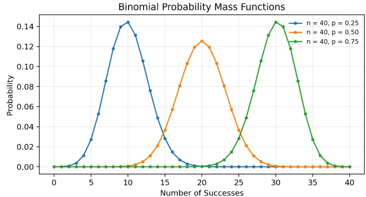
Figure 1 shows how the binomial distribution varies with the probability of success. With \(p = 0.50\), the distribution is balanced around the center. As \(p\) moves away from 0.50, the distribution becomes more asymmetric because most outcomes shift toward either fewer or more successes. The figure is useful because it shows why the same formula for variance, \(np(1 – p)\), depends on both the number of trials and the balance between success and failure probabilities.

Example 2: Profitable Signals from an Algorithmic Strategy

A quant researcher tests an intraday signal that has a 54% probability of producing a profitable trade. The strategy is expected to generate 120 independent trades next week. Assume each trade is classified simply as profitable or unprofitable.

Calculate the expected number of profitable trades, the variance, and the standard deviation.

Solution

We know that:

$$
\begin{align}
\mu = np
\end{align}
$$

$$
\begin{align}
\sigma^2 = np(1 – p)
\end{align}
$$

The expected number of profitable trades is:

$$
\begin{align}
\mu = 120 \times 0.54 = 64.8
\end{align}
$$

The variance is:

$$
\begin{align}
\sigma^2 = 120 \times 0.54 \times (1 – 0.54) = 29.808
\end{align}
$$

The standard deviation is:

$$
\begin{align}
\sigma = \sqrt{29.808} = 5.46
\end{align}
$$

The interpretation is not that exactly 64.8 trades will be profitable. The result means that, over many comparable weeks, the average number of profitable trades would be about 64.8, with meaningful variation around that average. Because \(np = 64.8\) and \(n(1 – p) = 55.2\), a normal approximation would be reasonable in this example.

Poisson Distribution

The Poisson distribution models the number of events occurring over a fixed interval of time or space when the events occur independently at a constant average rate. It is especially useful for rare event counts, such as defaults in a credit portfolio, cyber incidents, operational loss events, order arrivals, or liquidity withdrawals over a fixed period.

The probability of observing \(k\) events over an interval of length \(t\) is:

$$
\begin{align}
P(K = k) = \frac{(\lambda t)^k}{k!}e^{-\lambda t}
\end{align}
$$

Where:

• \(P(K = k)\) is the probability of observing exactly \(k\) events
• \(K\) is the random variable representing the number of events
• \(k\) is the specific number of events observed
• \(\lambda\) is the expected number of events per unit of time
• \(t\) is the length of the interval
• \(\lambda t\) is the expected number of events over the full interval
• \(k!\) is \(k\) factorial
• \(e\) is the base of the natural logarithm

For one unit of time, the mean and variance are:

$$
\begin{align}
\mu = \sigma^2 = \lambda
\end{align}
$$

Where:

• \(\mu\) is the mean number of events per unit of time.
• \(\sigma^2\) is the variance of the number of events per unit of time.
• \(\lambda\) is the event rate per unit of time.

For an interval of length \(t\), the corresponding mean and variance are \(\lambda t\). The equality of the mean and variance is a defining feature of the Poisson distribution.

The skewness and excess kurtosis are:

$$
\begin{align}
\text{Skewness} = \frac{1}{\sqrt{\lambda}}
\end{align}
$$

$$
\begin{align}
\text{Excess kurtosis} = \frac{1}{\lambda}
\end{align}
$$

Where:

• \(\lambda\) is the event rate over the relevant interval
• Skewness measures asymmetry
• Excess kurtosis measures tail heaviness relative to the normal distribution

As \(\lambda\) increases, skewness and excess kurtosis decline. In plain language, a Poisson distribution with a very low event rate is more visibly right-skewed, while a Poisson distribution with a higher event rate becomes more balanced.

Figure 2: Poisson Probability Mass Functions

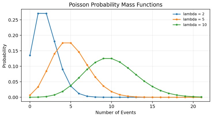
Figure 2 shows why the Poisson distribution is closely associated with rare events. When \(\lambda\) is low, most probability is concentrated near zero, and the distribution has a long right tail. As \(\lambda\) increases, the center of the distribution shifts to the right and the shape becomes less asymmetric. In risk management, that change matters: a portfolio with a higher expected number of events has a different distribution of event counts, not simply a larger average.

Example 3: Default Arrivals in a Private Credit Portfolio

A private credit portfolio has an estimated default intensity of 0.04 per year. Defaults are assumed to follow a Poisson process. Calculate the probability of observing exactly two defaults over a three‑year horizon.

Solution

We know that:

$$
\begin{align}
P(K = k) = \frac{(\lambda t)^k}{k!}e^{-\lambda t}
\end{align}
$$

For this case, \(\lambda = 0.04\), \(t = 3\), and \(k = 2\). The expected number of defaults over three years is:

$$
\begin{align}
\lambda t = 0.04 \times 3 = 0.12
\end{align}
$$

The probability of exactly two defaults is:

$$
\begin{align}
P(K = 2) = \frac{(0.12)^2}{2!}e^{-0.12} = 0.0064
\end{align}
$$

The probability is about 0.64%. The result is low because the expected number of defaults over the three years is only 0.12. The same model would produce a much higher probability if the portfolio had a higher intensity rate or a longer horizon.

For default intensity, analysts often also calculate the probability of at least one default:

$$
\begin{align}
P(K \geq 1) = 1 – e^{-\lambda t}
\end{align}
$$

Where:

• \(P(K \geq 1)\) is the probability of at least one event
• \(\lambda\) is the event rate per unit of time
• \(t\) is the length of the interval
• \(e^{-\lambda t}\) is the probability of zero events over the interval

In this example:

$$
\begin{align}
P(K \geq 1) = 1 – e^{-0.12} = 0.1131
\end{align}
$$

Thus, the probability of at least one default over three years is about 11.31%.

Continuous Uniform Distribution

A continuous uniform distribution applies when all values within an interval \([a, b]\) are equally likely. It is conceptually simple but very useful in simulation work. For example, many Monte Carlo models begin by drawing random numbers from a uniform distribution and then transforming those values into draws from another target distribution.

The mean is:

$$
\begin{align}
\mu = \frac{a+b}{2}
\end{align}
$$

This formula has already been defined for the discrete uniform distribution. The same expression gives the midpoint of a continuous interval.

The variance is:

$$
\begin{align}
\sigma^2 = \frac{(b-a)^2}{12}
\end{align}
$$

Where:

• \(\sigma^2\) is the variance of the continuous uniform distribution
• \(a\) is the lower bound of the interval
• \(b\) is the upper bound of the interval
• \(b – a\) is the width of the interval

The continuous uniform distribution has skewness of 0 and kurtosis of 1.8, which means its excess kurtosis is \(1.8 – 3 = -1.2\). Compared with the normal distribution, its tails are lighter.

Example 4: Random Shock in a Liquidity Simulation

A liquidity analyst models a one‑day deposit‑flow shock as uniformly distributed between –2.0% and +2.0% of deposits.

Calculate the mean, variance, and standard deviation of the shock.

Solution

Recall that:

$$
\begin{align}
\mu = \frac{a+b}{2}
\end{align}
$$

$$
\begin{align}
\sigma^2 = \frac{(b-a)^2}{12}
\end{align}
$$

The mean shock is:

$$
\begin{align}
\mu = \frac{-2.0+2.0}{2} = 0.0\%
\end{align}
$$

The variance is:

$$
\begin{align}
\sigma^2 = \frac{(2.0-(-2.0))^2}{12} = \frac{16}{12} = 1.3333
\end{align}
$$

The standard deviation is:
$$
\sigma – \sqrt{1.3333} = 1.15\% $$

The mean shock is zero because the interval is symmetric around zero. The standard deviation captures the uncertainty introduced by allowing shocks to fall anywhere between -2.0% and +2.0%.

Normal Distribution

The normal distribution is a continuous, symmetric, bell-shaped distribution. It is fully described by its mean and variance and is denoted as:

$$
X \sim N(\mu, \sigma^2)
$$

Where:

• \(X\) is the normally distributed random variable
• \(N(\mu, \sigma^2)\) denotes a normal distribution
• \(\mu\) is the mean
• \(\sigma^2\) is the variance

For the normal distribution, the mean, median, and mode are equal. The skewness is 0, the kurtosis is 3, and the excess kurtosis is 0. These properties make the normal distribution very convenient for modeling and statistical inference.

The normal distribution is widely used in finance, but it must be used with judgment. Daily returns may appear roughly normal during quiet periods, but real-world financial returns can exhibit skewness, volatility clustering, and fat tails. A normal model may therefore understate the likelihood of extreme outcomes if the actual return process is more turbulent than the model assumes.

Example 5: Interpreting Normal Return Distribution

An analyst models the monthly return of a low‑volatility equity strategy as normally distributed with a mean of 0.70% and a standard deviation of 2.20%.

Calculate the variance and the one‑standard‑deviation range of returns.

Solution

We know that:

$$
X \sim N(\mu, \sigma^2)
$$

The variance is:

$$
\sigma^2 = (2.20)^2 = 4.84
$$

The one-standard-deviation range is:

$$
\mu \pm \sigma = 0.70\% \pm 2.20\%
$$

Therefore:

$$
– 1.50\% \leq X \leq 2.90\%
$$

For a normal distribution, approximately 68% of observations fall within one standard deviation of the mean. The analyst would therefore expect about 68% of monthly returns to fall between -1.50% and 2.90%, assuming the normal model is appropriate.

Log-Normal Distribution

A variable is log-normally distributed if its logarithm is normally distributed. This distribution is especially important in finance because asset prices cannot be negative. Stock prices, certain commodity prices, and other non-negative quantities are often better modeled with a log-normal distribution than with a normal distribution.

If \(X\) is normally distributed and \(Y = e^X\), then \(Y\) is log-normally distributed. Its mean is:

$$
\mu_Y = e^{\mu_X + \frac{\sigma_X^2}{2}}
$$

Where:

• \(\mu_Y\) is the mean of the log-normally distributed variable \(Y\)
• \(Y\) is the log-normally distributed variable
• \(X\) is the normally distributed logarithm of \(Y\)
• \(\mu_X\) is the mean of \(X\)
• \(\sigma_X^2\) is the variance of \(X\)
• \(e\) is the base of the natural logarithm

The variance is:

$$
\sigma_Y^2 = \left(e^{\sigma_X^2} – 1\right) e^{2\mu_X + \sigma_X^2}
$$

Where:

• \(\sigma_Y^2\) is the variance of the log-normally distributed variable \(Y\)
• \(\sigma_X^2\) is the variance of \(X\)
• \(\mu_X\) is the mean of \(X\)

A log-normal distribution is right-skewed. This is a natural feature of asset prices: the price cannot fall below zero, but very large positive values are possible.

For price modeling under continuously compounded returns, a commonly used expression is:

$$
\ln(S_T) = \ln(S_0) + \left(\mu – \frac{\sigma^2}{2}\right)T
$$

Where:

• \(S_T\) is the modeled price at time \(T\)
• \(S_0\) is the current price
• \(\mu\) is the mean continuously compounded return
• \(\sigma^2\) is the variance of continuously compounded returns
• \(T\) is the time horizon
• \(\ln(\cdot)\) denotes the natural logarithm

The term \(-\sigma^2 / 2\) is sometimes called the volatility adjustment. Easy to miss, it’s a common source of incorrect answers in exam questions.

Figure 3: Normal, Log-normal, and Logistic Distributions

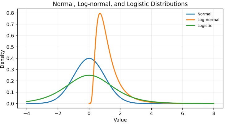
Figure 3 compares three continuous distributions. The normal distribution is symmetric and centered around its mean. The log-normal distribution is right-skewed and begins at positive values, making it useful for modeling asset prices. The logistic distribution is also symmetric, but it has heavier tails than the normal distribution. This visual comparison helps candidates avoid a common mistake: assuming that every bell-shaped curve behaves like a normal distribution.

Example 6: Modeling a Non-Negative Asset Price

A stock currently trades at USD80. An analyst assumes that the continuously compounded annual return has a mean of 7% and a standard deviation of 25%. Estimate the expected price level after one year using the log-normal price relationship.

Solution

Recall that:

$$
\ln(S_T) = \ln(S_0) + \left(\mu – \frac{\sigma^2}{2}\right)T
$$

Substitute the inputs:

$$
\begin{align}
\ln(S_1) &= \ln(80) + \left(0.07 – \frac{0.25^2}{2}\right)(1) \\
\ln(S_1) &= 4.3820 + (0.07 – 0.03125) = 4.4208
\end{align}
$$

Now exponentiate both sides:

$$
S_1 = e^{4.4208} = 83.16
$$

The modeled one-year price is approximately USD83.16. The result is positive by construction, which is one reason the log-normal distribution is preferred for modeling price levels.

Logistic Distribution

The logistic distribution is a continuous distribution with a symmetric shape and an S-shaped cumulative distribution function. It is especially important in logistic regression, which is used for binary classification problems. In finance, a model might estimate whether a borrower defaults or does not default, whether a client churns or does not churn, or whether a transaction is flagged as suspicious or not suspicious.

The logistic distribution is defined by a location parameter and a scale parameter. Its mean is:

$$
\mu = \mu
$$

Where:

• The \(\mu\) on the left is the mean of the logistic distribution.
• The \(\mu\) on the right is the location parameter.

Its variance is:

$$
\sigma^2 = \frac{s^2 \pi^2}{3}
$$

Where:

• \(\sigma^2\) is the variance of the logistic distribution
• \(s\) is the scale parameter
• \(\pi\) is the mathematical constant pi

The logistic distribution has a skewness of 0, a kurtosis of 4.2, and an excess kurtosis of 1.2. The positive excess kurtosis means that its tails are heavier than those of the normal distribution.

Example 7: Logistic Scale and Variance

A model validation team compares two logistic classification models. Model A has a scale parameter \(s = 1.0\), and Model B has a scale parameter \(s = 1.5\). Compare the variances of the two underlying logistic distributions.

Solution

Start by quoting the formula:

$$
\sigma^2 = \frac{s^2 \pi^2}{3}
$$

For Model A:

$$
\sigma_A^2 = \frac{1.0^2 \pi^2}{3} = 3.29
$$

For Model B:

$$
\sigma_B^2 = \frac{1.5^2 \pi^2}{3} = 7.40
$$

The variance increases with the square of the scale parameter. Increasing \(s\) from 1.0 to 1.5 does not increase variance by 50%; it increases variance by 125%. This is exactly the kind of detail that can turn a concept question into a calculation question.

Summary of Principal Moments

$$ \textbf{Table 3: Mean and Variance of Key Distributions} \\
\begin{array}{l|c|c}
\textbf{Distribution} & \textbf{Mean} & \textbf{Variance} \\
\hline
\text{Discrete uniform} & \frac{a + b}{2} & \frac{(b – a + 1)^2 – 1}{12} \\
\hline
\text{Binomial} & np & np(1 – p) \\
\hline
\text{Poisson} & \lambda & \lambda \\
\hline
\text{Continuous uniform} & \frac{a + b}{2} & \frac{(b – a)^2}{12} \\
\hline
\text{Normal} & \mu & \sigma^2 \\
\hline
\text{Log-normal} & e^{\mu + \frac{\sigma^2}{2}} & \left(e^{\sigma^2} – 1\right)e^{2\mu + \sigma^2} \\
\hline
\text{Logistic} & \mu & \frac{s^2 \pi^2}{3} \\
\end{array}
$$

$$ \textbf{Table 4: Skewness and Excess Kurtosis of Key Distributions} \\
\begin{array}{l|c|c}
\textbf{Distribution} & \textbf{Skewness} & \textbf{Excess Kurtosis} \\ \hline
\text{Discrete uniform} & 0 & { – \frac {6(n^2+1)}{5(n^2-1)} } \\ \hline
\text{Binomial} & \frac {(1-2p)}{\sqrt{np(1-p)}} & \frac {(1-6p(1-p))}{(np(1-p))} \\ \hline
\text{Poisson} & \frac {1}{\sqrt{\lambda}} & \frac {1}{{\lambda}} \\ \hline
\text{Continuous uniform} & 0 & \frac{-6}{5} \\ \hline
\text{Normal} & 0 & 0 \\ \hline
\text{Log-normal} & \text{Positive} & \text{Positive} \\ \hline
\text{Logistic} & 0 & 1.2
\end{array} $$

Tables 3 and 4 pull the learning outcome together. The mean and variance are usually the most tested calculations, but the interpretation of skewness and excess kurtosis is just as important. A right-skewed distribution suggests a long right tail; positive excess kurtosis suggests heavier tails than a normal distribution. These are not abstract statistics. They determine whether a model might understate rare losses, overstate symmetry, or apply the wrong logic to asset prices.

Interpretation and Evaluation

The binomial distribution is appropriate for the number of profitable trades only if each trade can reasonably be treated as an independent success-or-failure trial with a stable success probability. The Poisson distribution is appropriate for rare event counts only if events arrive independently at a reasonably stable rate. The normal distribution is useful for many approximations, but it can be problematic when modeling variables that cannot be negative or when the data exhibit heavy-tailed behavior. The log-normal distribution solves the non-negative price problem, but it may still be too simple when prices jump or volatility changes over time. The logistic distribution is powerful in classification problems, but its heavier tails must be understood when comparing it with a normal model.

Good financial work, therefore, requires both computation and judgment. The formula gives the number; the model choice gives that number meaning.

Question

A credit analyst models default arrivals in a diversified private credit portfolio as a Poisson process with an annual default intensity of 0.025. The analyst evaluates a four-year horizon.

Which of the following is closest to the probability of at least one default over the four-year horizon and the corresponding mean and variance of the number of defaults over that horizon?

1. 9.52%; mean = 0.10; variance = 0.10
2. 9.52%; mean = 0.025; variance = 0.025
3. 9.048%; mean = 0.10; variance = 0.10

The correct answer is A.

$$
\begin{align}
P(K \geq 1) &= 1 – e^{-\lambda t} \\
\mu = \sigma^2 &= \lambda t
\end{align}
$$

Where:

• \(P(K \geq 1)\) is the probability of at least one event
• \(K\) is the random variable representing the number of defaults
• \(\lambda\) is the annual default intensity
• \(t\) is the time horizon in years
• \(e\) is the base of the natural logarithm
• \(\mu\) is the mean number of defaults over the horizon
• \(\sigma^2\) is the variance of the number of defaults over the horizon
• \(\lambda t\) is the expected number of defaults over the full horizon

First, calculate the expected number of defaults over four years:

$$
\lambda t = 0.025 \times 4 = 0.10
$$

For a Poisson distribution over the full interval:

$$
\mu = \sigma^2 = 0.10
$$

Now calculate the probability of at least one default:

$$
P(K \geq 1) = 1 – e^{-0.10} = 1 – 0.9048 = 0.0952
$$

The probability of at least one default is therefore 9.52%, and the mean and variance of the number of defaults over the horizon are both 0.10.

B is incorrect because it uses the annual intensity, 0.025, as if it were the four-year mean and variance. The mean and variance must be based on \(\lambda t\), not \(\lambda\) alone, when the horizon is longer than one year.

C is incorrect because it gives the probability of zero defaults, \(e^{-0.10} = 90.48\%\), rather than the probability of at least one default.