Parametric vs Non-Parametric Tests: When to Use Each in Financial Analysis

Why the Choice of Test Matters

A hypothesis test is only as useful as the assumptions behind it. A polished t-statistic, p-value, or critical-value comparison can look authoritative even when the test is poorly matched to the data. The analyst therefore has to make a judgment before calculation begins: Is this a setting in which a parametric test is appropriate, or is a non-parametric test the better tool?

Parametric tests rely on assumptions about the population distribution or its parameters, such as the mean and variance. Non-parametric tests are less dependent on a specific distributional form and are often useful when the data are ordinal, categorical, highly skewed, or contaminated by outliers.

This is not a contest in which one class of tests always wins. Parametric tests are often more powerful when their assumptions hold. Non-parametric tests are often more robust when those assumptions are doubtful. The professional task is to match the method to the data and to interpret the evidence without overstating what the test can prove.

Parametric and Non-Parametric Tests Compared

A parametric test uses assumptions about a population distribution and tests hypotheses about population parameters. Examples include t-tests for means, chi-square tests for a single population variance, F-tests for comparing variances, and Pearson correlation tests.

A non-parametric test does not require the same distributional assumptions. It may use ranks, categories, counts, or signs rather than the raw values themselves. The Spearman rank correlation test and the chi-square test of independence for categorical data are central examples in this learning outcome.

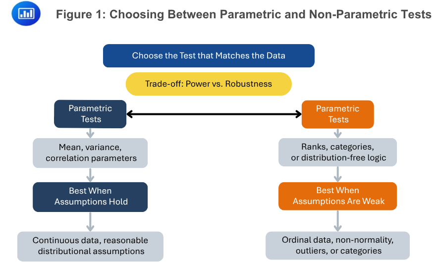
Figure 1 frames the decision. Parametric tests are preferred when the measurement scale, sample design, distributional assumptions, and variance assumptions are reasonable. Non-parametric tests become attractive when those requirements are not credible, especially with ranks, categories, non-normal data, small samples, or influential outliers.

$$ \textbf{Table 1: Parametric and Non-Parametric Tests Compared} \\
\begin{array}{l|l|l}
\textbf{Feature} & \textbf{Parametric Tests} & \textbf{Non-Parametric Tests} \\
\hline
\text{Core input} & \text{Raw numerical observations and} & \text{Ranks, signs, categories, counts,} \\
& \text{distributional parameters} & \text{or distribution-free statistics} \\ \hline
\text{Typical assumptions} & \text{Known or assumed distribution,} & \text{Fewer distributional assumptions;} \\
& \text{often normality; interval or ratio data} & \text{useful for ordinal or categorical data} \\
\hline
\text{Power when assumptions hold} & \text{Usually higher} & \text{Often lower than the corresponding} \\
& & \text{parametric test} \\ \hline
\text{Robustness when assumptions fail} & \text{Can be misleading} & \text{Usually more robust} \\
\hline
\text{Common examples} & \text{t-test, F-test, Pearson correlation} & \text{Spearman rank correlation test,} \\
& \text{test} & \text{chi-square test of independence}
\end{array}
$$

Table 1 gives the practical trade-off. A non-parametric test is not automatically more accurate. It is more flexible and robust in difficult data settings, but a well-specified parametric test may detect true effects more efficiently when the parametric assumptions are satisfied.

When Each Type of Test is More Appropriate

A parametric test is usually appropriate when the variable is measured on an interval or ratio scale, the sample is reasonably large, or the population is approximately normal, the observations are independent, and the relevant assumptions about variance are credible. For example, testing whether the mean monthly return of a liquid index differs from zero can often be handled with a parametric test if the sample is large and the return process is not dominated by extreme outliers.

A non-parametric test is usually more appropriate when the variable is ordinal, when the distribution is strongly non-normal, when outliers could dominate the estimate, or when the data are categorical counts. For example, testing whether fund size classifications are independent of investment-style classifications is naturally a chi-square test of independence, not a t-test, because the data are counts in categories rather than continuous returns.
$$
\begin{array}{l|l|l}
\textbf{Situation} & \textbf{More Appropriate Test Type} & \textbf{Reason} \\
\hline
\text{Monthly excess returns are} & \text{Parametric} & \text{The test concerns a population} \\
\text{approximately normal and the} & & \text{parameter and assumptions are} \\
\text{question concerns a mean} & & \text{plausible} \\
\hline
\text{ESG ratings are grouped as} & \text{Non-parametric} & \text{The data are categorical or ordinal} \\
\text{progressive, average, or poor} & & \\
\hline
\text{A dataset contains severe} & \text{Non-parametric} & \text{Rank-based or count-based} \\
\text{skewness and influential outliers} & & \text{methods may be more robust} \\
\hline
\text{The analyst compares variances} & \text{Parametric} & \text{An F-test directly addresses the} \\
\text{from two normally distributed return} & & \text{variance comparison} \\
\text{series} & & \\
\hline
\text{The analyst tests whether two} & \text{Non-parametric} & \text{A chi-square test uses observed} \\
\text{classifications are independent} & & \text{and expected frequencies}
\end{array}
$$

Table 2 is a useful exam guide. The word appropriate is important. A test is appropriate when its logic matches the data, the hypothesis, and the assumptions.

Example 1: Selecting the Correct Type of Test

Imagine an analyst is studying whether the liquidity bucket assigned to a corporate bond is related to its credit-rating bucket. Liquidity is classified as high, medium, or low. Credit quality is classified as investment grade, crossover, or high yield. The analyst has a table of counts for 600 bonds.

The objective is to choose the right test. A parametric mean test would not be appropriate because the data are not raw numerical returns. They are categorical classifications. The appropriate approach is a non-parametric chi-square test of independence because the analyst wants to test whether the two categorical variables are independent.

The correct hypotheses would be:

$$
\begin{array}{l}
H_0: \text{Liquidity bucket and credit-rating bucket are independent} \\
H_a: \text{Liquidity bucket and credit-rating bucket are not independent}
\end{array}
$$

The conclusion should be phrased carefully. If the null is rejected, the analyst may conclude that there is evidence of an association between the classifications. The test does not prove that credit rating causes liquidity or that liquidity causes credit rating.

Spearman Rank Correlation

Pearson correlation measures a linear relationship between two variables. Spearman rank correlation measures the degree to which two variables move together in a monotonic relationship. A monotonic relationship means that as one variable increases, the other tends to consistently increase or consistently decrease, even if the relationship is not linear.

Spearman rank correlation is calculated using ranks rather than raw values. Each variable is ranked from smallest to largest, the rank differences are calculated for each paired observation, and those differences are used to calculate the correlation coefficient.

When there are no tied ranks, the Spearman rank correlation coefficient is:

$$
r_s = 1 – \frac{6 \sum_{i=1}^{n} d_i^2}{n(n^2 – 1)}
$$

Where:

• \( r_s \) is the Spearman rank correlation coefficient
• \( d_i \) is the difference between the two ranks for paired observation \( i \)
• \( d_i^2 \) is the squared rank difference for paired observation \( i \)
• \( n \) is the number of paired observations
• \( \sum_{i=1}^{n} d_i^2 \) is the sum of squared rank differences

If there are tied values, average ranks are assigned to tied observations. In practice, when ties are present, analysts often compute the Pearson correlation on the ranked data.

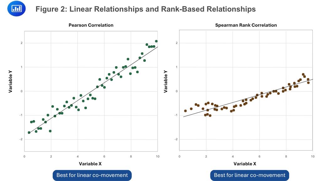
Figure 2 shows the key distinction. Pearson correlation is most natural when the relationship is linear. Spearman rank correlation is useful when the relationship is monotonic but not necessarily linear. In finance, this can matter when raw observations are skewed, capped, floored, or distorted by extreme values.

Example 2: Calculating Spearman Rank Correlation

Assume we have five private-market funds ranked by due-diligence score and by subsequent one-year performance rank. We want to know whether higher due-diligence scores were associated with stronger performance rankings.

$$\begin{array}{l|c|c|c|c}
\textbf{Fund} & \textbf{Due-Diligence Rank} & \textbf{Performance Rank} & \textbf{Difference, } d_i & \textbf{Squared Difference, } d_i^2 \\
\hline
\text{A} & 1 & 2 & -1 & 1 \\\hline
\text{B} & 2 & 1 & 1 & 1 \\\hline
\text{C} & 3 & 4 & -1 & 1 \\\hline
\text{D} & 4 & 3 & 1 & 1 \\\hline
\text{E} & 5 & 5 & 0 & 0 \\\hline
\text{Total} & & & & 4
\end{array}
$$

Solution

Recall:

$$
r_s = 1 – \frac{6 \sum_{i=1}^{n} d_i^2}{n(n^2 – 1)}
$$

Where:

• \( r_s \) is the Spearman rank correlation coefficient
• \( n = 5 \) is the number of paired fund observations
• \( d_i \) is the difference between the due-diligence rank and performance rank for fund \( i \)
• \( \sum_{i=1}^{n} d_i^2 = 4 \) is the sum of squared rank differences

Substitute the values:

$$\begin{align}r_s& = 1 – \frac{6(4)}{5(5^2 – 1)}\\&= 1 – \frac{24}{120} = 0.80\end{align}$$

The Spearman rank correlation is 0.80. This indicates a strong positive rank association in this small sample. Funds with better due-diligence ranks tended to have better performance ranks. The result should still be interpreted cautiously because the sample contains only five funds.

Testing Spearman Rank Correlation

The null hypothesis in a Spearman rank correlation test usually states that the population rank correlation is zero:

$$
\begin{array}{l}
H_0: \rho_s = 0 \\
H_A: \rho_s \neq 0
\end{array}
$$

For large samples, the test statistic can be approximated with a t-distribution:

$$
t = \frac{r_s \sqrt{n-2}}{\sqrt{1-r_s^2}}
$$

Where:

• \( t \) is the test statistic
• \( r_s \) is the sample Spearman rank correlation coefficient
• \( n \) is the number of paired observations
• \( n – 2 \) is the degrees of freedom

For small samples, specialized critical-value tables are typically used. For larger samples, the t-approximation becomes more practical.

Example 3: Testing a Spearman Rank Correlation

Let’s say an analyst evaluates 42 emerging-market ETFs. The analyst ranks each ETF by expense ratio and by three-year active return, then calculates a Spearman rank correlation of -0.36. The analyst wants to test whether the rank relationship differs from zero at the 5% significance level using a two-tailed test. The 5% two-tailed critical value is approximately ±2.02.

Solution

We know that:

$$
t = \frac{r_s \sqrt{n-2}}{\sqrt{1-r_s^2}}
$$

Where:

• \( t \) is the test statistic for the Spearman rank correlation
• \( r_s = -0.36 \) is the sample Spearman rank correlation
• \( n = 42 \) is the number of ETF observations
• \( n – 2 = 40 \) is the degrees of freedom

Substituting the values:

$$\begin{align}t&= \frac{-0.36 \sqrt{42 – 2}}{\sqrt{1 – (-0.36)^2}}\\&=
\frac{-0.36 \sqrt{40}}{\sqrt{0.8704}} = -2.44\end{align}$$

Because \(|t| = 2.44 \) exceeds 2.02, the analyst rejects the null hypothesis at the 5% significance level. There is evidence of a statistically significant monotonic relationship between expense-ratio rank and three-year active-return rank. The negative sign indicates that higher expense-ratio ranks are associated with lower active-return ranks in this sample.

Chi-Square Test of Independence

A chi-square test of independence is used when the data are classified into categories across two dimensions. The test compares observed frequencies with expected frequencies that would be expected if the two classifications were independent.

The expected frequency for cell \( (i, j) \) is:

$$
E_{ij} = \frac{(\text{Row Total}_i)(\text{Column Total}_j)}{N}
$$

Where:

• \( E_{ij} \) is the expected frequency in row \( i \) and column \( j \)
• \( \text{Row Total}_i \) is the total number of observations in row \( i \)
• \( \text{Column Total}_j \) is the total number of observations in column \( j \)
• \( N \) is the total number of observations

The chi-square test statistic is:

$$
\chi^2 = \sum_{i=1}^{r} \sum_{j=1}^{c} \frac{(O_{ij} – E_{ij})^2}{E_{ij}}
$$

Where:

• \( \chi^2 \) is the chi-square test statistic
• \( O_{ij} \) is the observed frequency in row \( i \) and column \( j \)
• \( E_{ij} \) is the expected frequency in row \( i \) and column \( j \)
• \( r \) is the number of rows
• \( c \) is the number of columns

The degrees of freedom for the chi-square test of independence are:

$$
df = (r – 1)(c – 1)
$$

Where:

• \( df \) is the degrees of freedom
• \( r \) is the number of rows in the contingency table
• \( c \) is the number of columns in the contingency table

Because the squared deviations cannot be negative, the rejection region is in the right tail. A larger chi-square statistic indicates a larger gap between observed and expected frequencies and therefore stronger evidence against independence.

Figure 3: Chi-Square Test of Independence: Right-Tailed Decision Rule

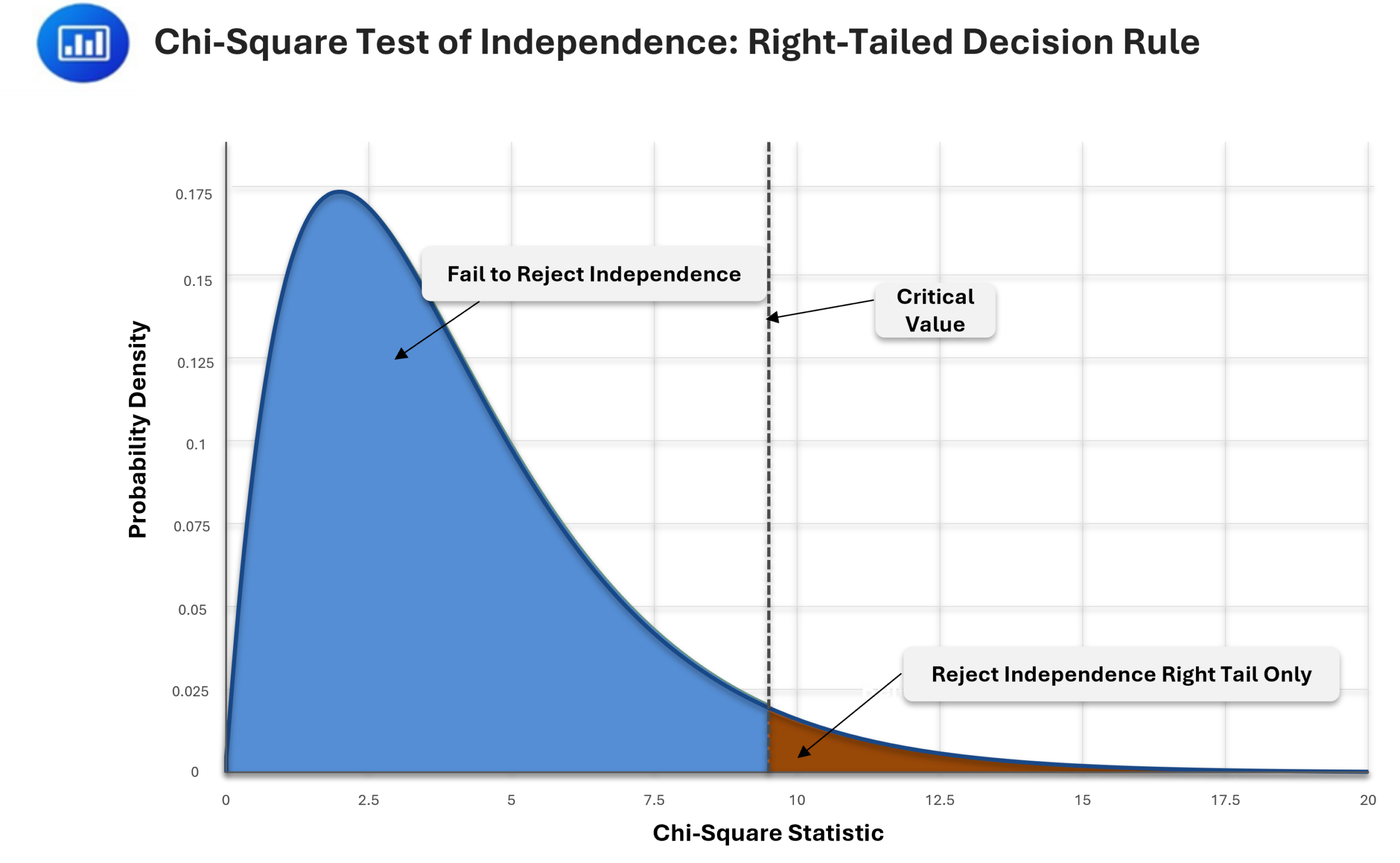
Figure 3 shows why the chi-square test of independence has a right-tailed decision rule. When observed and expected frequencies are very similar, the test statistic is small. As the gaps between observed and expected frequencies become larger, the statistic moves into the right tail, where the null hypothesis of independence may be rejected.

Example 4: Constructing and Interpreting a Chi-Square Test of Independence

Consider a sample of 300 listed companies classified by board diversity score and cyber-risk disclosure quality. The analyst wants to test whether the two classifications are independent at the 5% significance level.

$$
\begin{array}{l|c|c|c|c}
{\textbf{Board Diversity}\\ \textbf{Score}} & {\textbf{Strong} \\ \textbf{Disclosure}} & {\textbf{Moderate} \\ \text{Disclosure}} & {\textbf{Weak} \\ \textbf{Disclosure}} & {\textbf{Row} \\ \textbf{Total}} \\
\hline
\text{High} & 42 & 30 & 18 & 90 \\ \hline
\text{Medium} & 34 & 56 & 30 & 120 \\ \hline
\text{Low} & 14 & 34 & 42 & 90 \\ \hline
\text{Column Total} & 90 & 120 & 90 & 300
\end{array}
$$

Solution

The hypotheses are:

$$
\begin{array}{l}
H_0: \text{Board diversity score and cyber-risk disclosure quality are independent} \\
H_A: \text{Board diversity score and cyber-risk disclosure quality are not independent}
\end{array}
$$

Start with the expected-frequency formula:

$$
E_{ij} = \frac{(\text{Row Total}_i)(\text{Column Total}_j)}{N}
$$

Where:

• \( E_{ij} \) is the expected frequency in row \( i \) and column \( j \)
• \( N = 300 \) is the total number of companies
• \( \text{Row Total}_i \) is the row total for board diversity category \( i \)
• \( \text{Column Total}_j \) is the column total for disclosure quality category \( j \)

For the high-diversity and strong-disclosure cell:

$$
E_{11} = \frac{(90)(90)}{300} = 27
$$

The expected frequencies are:

$$
\begin{array}{l|c|c|c}
{\textbf{Board Diversity} \\ \textbf{Score} }& {\textbf{Strong} \\ \textbf{Disclosure}} & {\textbf{Moderate} \\ \textbf{Disclosure}} & {\textbf{Weak} \\ \textbf{Disclosure}} \\
\hline
\text{High} & 27 & 36 & 27 \\ \hline
\text{Medium} & 36 & 48 & 36 \\ \hline
\text{Low} & 27 & 36 & 27
\end{array}
$$

Now quote the chi-square statistic:

$$
\chi^2 = \sum_{i=1}^{r} \sum_{j=1}^{c} \frac{(O_{ij} – E_{ij})^2}{E_{ij}}
$$

Where:

• \( O_{ij} \) is the observed frequency in row \( i \) and column \( j \)
• \( E_{ij} \) is the expected frequency in row \( i \) and column \( j \)
• \( r = 3 \) is the number of board-diversity categories
• \( c = 3 \) is the number of disclosure-quality categories

The scaled squared deviations are:

$$\begin{array}{l|c|c|c}
{\textbf{Board Diversity}\\ \textbf{Score}} & {\textbf{Strong} \\ \textbf{Disclosure}} & {\textbf{Moderate} \\ \textbf{Disclosure}} & {\textbf{Weak} \\ \textbf{Disclosure}} \\\hline
\text{High} & 8.33 & 1.00 & 3.00 \\ \hline
\text{Medium} & 0.11 & 1.33 & 1.00 \\ \hline
\text{Low} & 6.26 & 0.11 & 8.33
\end{array}$$

Summing the scaled squared deviations gives:

$$
\chi^2 = 29.47
$$

The degrees of freedom are:

$$
df = (r – 1)(c – 1) = (3 – 1)(3 – 1) = 4
$$

At the \( 5\% \) significance level with \( 4 \) degrees of freedom, the critical value is approximately \( 9.49 \). Because \( 29.47 \) is greater than \( 9.49 \), the analyst rejects the null hypothesis of independence. There is evidence that board diversity score and cyber-risk disclosure quality are related in this sample.

Standardized Residuals

A chi-square test can tell us whether two classifications appear to be related, but it does not immediately tell us which cells are driving the result. Standardized residuals help identify where the largest differences between observed and expected frequencies occur.

The standardized residual is:

$$
\text{Standardized Residual}_{ij} = \frac{O_{ij} – E_{ij}}{\sqrt{E_{ij}}}
$$

Where:

• \( \text{Standardized Residual}_{ij} \) is the standardized residual for row \( i \) and column \( j \)
• \( O_{ij} \) is the observed frequency in row \( i \) and column \( j \)
• \( E_{ij} \) is the expected frequency in row \( i \) and column \( j \)
• \( E_{\sqrt{ij}} \) is the square root of the expected frequency

A large positive residual means the observed count is meaningfully higher than expected under independence. A large negative residual means the observed count is meaningfully lower than expected. As a practical rule, residuals with magnitudes greater than about 1.96 may be treated as notable at an approximate 5% level.

Example 5: Interpreting Standardized Residuals

Now imagine we want to identify the cells driving the chi-square result in Example 4. For the high-diversity and strong-disclosure cell, the observed frequency is 42 and the expected frequency is 27.

Solution

We use the formula:

$$
\text{Standardized Residual}_{11} = \frac{O_{11} – E_{11}}{\sqrt{E_{11}}}
$$

Where:

• \( O_{11} = 42 \) is the observed number of high-diversity firms with strong disclosure
• \( E_{11} = 27 \) is the expected number of such firms under independence
• \( \text{Standardized Residual}_{11} \) is the standardized residual for the high-diversity and strong-disclosure cell

Substituting the values:

$$
\text{Standardized Residual}_{11} = \frac{42 – 27}{\sqrt{27}} = 2.89
$$

The residual is positive and larger than \( 1.96 \) in magnitude. This means high-diversity firms with strong cyber-risk disclosure occurred more often than expected if the two classifications were independent. This cell is one of the drivers of the overall rejection of independence.

Interpreting Results without Overclaiming

Non-parametric tests can be powerful safeguards against overconfidence, but they still require disciplined interpretation.

For Spearman rank correlation, rejecting the null hypothesis indicates evidence of a statistically significant monotonic association. It does not prove causation. It also does not guarantee that the relationship is economically meaningful.

For the chi-square test of independence, rejecting the null hypothesis indicates evidence that the two classifications are not independent. It does not identify a causal channel, and it does not say that every cell in the contingency table is important. Standardized residuals help locate the cells that contribute most to the result.

Analysts should also remember that non-parametric methods may be less powerful than parametric methods when parametric assumptions are valid. Robustness is valuable, but it comes with a trade-off.

Interpretation and Evaluation

Several practical summary follow:

• Parametric tests are usually more powerful when their assumptions hold.
• Non-parametric tests are often more robust when the data are ordinal, categorical, non-normal, or affected by outliers.
• Pearson correlation tests linear relationships; Spearman rank correlation tests monotonic rank relationships.
• The Spearman rank correlation formula uses paired ranks and squared rank differences.
• A chi-square test of independence compares observed frequencies with expected frequencies under independence.
• The chi-square test of independence has a right-tailed rejection region.
• Standardized residuals help identify which contingency-table cells drive a significant chi-square result.
• Statistical significance should not be interpreted as causation or as a complete investment recommendation.

Question

A researcher classifies 240 companies by sustainability disclosure quality and institutional ownership level. The observed frequencies are:

$$ \begin{array}{l|c|c|c}
\textbf{Sustainability Disclosure} & \textbf{High Ownership} & \textbf{Low Ownership} & \textbf{Row Total} \\
\hline
\text{Strong} & 70 & 30 & 100 \\ \hline
\text{Weak} & 50 & 90 & 140 \\ \hline
\text{Column Total} & 120 & 120 & 240
\end{array}$$

Find the chi-square test statistic for this data.

1. 13.71
2. 26.45
3. 27.43

The correct answer is C.

We know that:

$$
E_{ij} = \frac{(\text{Row Total}_i)(\text{Column Total}_j)}{N}
$$

Where:

• \( E_{ij} \) is the expected frequency in row \( i \) and column \( j \)
• \( \text{Row Total}_i \) is the row total for disclosure category \( i \)
• \( \text{Column Total}_j \) is the column total for ownership category \( j \)
• \( N = 240 \) is the total number of companies

The expected frequencies are:

$$
\begin{align}
E_{11} &= \frac{(100)(120)}{240} = 50 \\
E_{12} &= \frac{(100)(120)}{240} = 50 \\
E_{21} &= \frac{(140)(120)}{240} = 70 \\
E_{22} &= \frac{(140)(120)}{240} = 70
\end{align}
$$

Now using the chi-square statistic formula:

$$
\chi^2 = \sum_{i=1}^{r} \sum_{j=1}^{c} \frac{(O_{ij} – E_{ij})^2}{E_{ij}}
$$

Where:

• \( \chi^2 \) is the chi-square test statistic
• \( O_{ij} \) is the observed frequency in row \( i \) and column \( j \)
• \( E_{ij} \) is the expected frequency in row \( i \) and column \( j \)
• \( r = 2 \) is the number of rows
• \( c = 2 \) is the number of columns

Substitute the observed and expected frequencies:

$$
\begin{align}
\chi^2 &= \frac{(70-50)^2}{50} + \frac{(30-50)^2}{50} + \frac{(50-70)^2}{70} + \frac{(90-70)^2}{70} \\
&= 8.00 + 8.00 + 5.71 + 5.71 = 27.43
\end{align}
$$

The chi-square test statistic is approximately 27.43.