Minimum-Variance Portfolio and Efficient Frontier: Calculation and Interpretation

From Feasible Portfolios to Portfolio Choice

Once an analyst can calculate portfolio return and portfolio risk, the next question is more interesting: which portfolio should be chosen? A universe of available securities can be combined in many ways. Some combinations use conservative weights and produce moderate risk. Others concentrate in growth assets and produce higher expected returns with higher volatility. Many possible combinations are simply unattractive because another available portfolio offers a higher expected return for the same risk, or the same expected return with lower risk.

The set of all portfolios that can be formed from the available assets is called the feasible set. The feasible set depends on the assets being considered and on any constraints imposed on portfolio weights. A long-only investor, for example, normally requires all asset weights to be non-negative. A hedge fund may permit short positions, leverage, or derivatives exposure. A pension portfolio may have additional constraints on liquidity, credit quality, currency exposure, or ESG exclusions.

The aim of mean-variance analysis is to separate feasible portfolios that are efficient from those that are dominated. An efficient portfolio is not merely a portfolio with a high return. It is a portfolio that offers the best available return-risk trade-off within the feasible set.

Figure 1: Feasible Portfolios and the Efficient Frontier

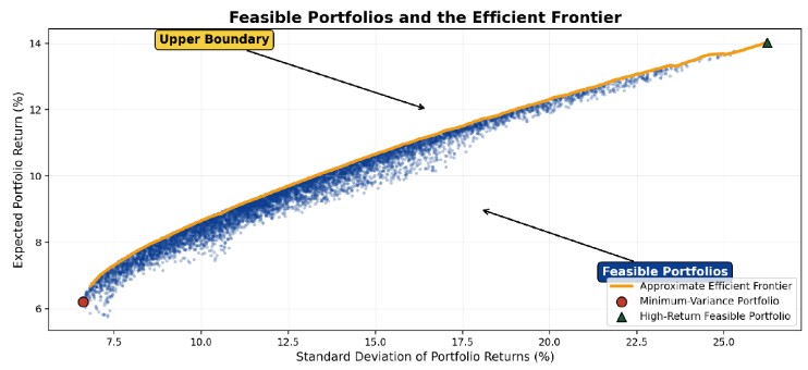
Figure 1 shows a simulated cloud of feasible portfolios built from four asset classes. Most points inside the cloud are not efficient because there is another portfolio above them with the same or similar risk but a higher expected return. The upper boundary is the efficient frontier. Portfolios above and to the left of the frontier would be desirable, but they are not available from the current investment opportunity set.

The Efficient Frontier

The efficient frontier is the set of portfolios that maximize expected return for each level of risk. Equivalently, it is the set of portfolios that minimize risk for each level of expected return. A portfolio below the efficient frontier is inefficient because at least one feasible portfolio offers a superior risk-return trade-off.

$$ \textbf{Table 1: Feasible, Inefficient, and Efficient Portfolios} \\
\begin{array}{l|l|l}
\textbf{Portfolio Type} & \textbf{Description} & \textbf{Practical Interpretation} \\
\hline
\text{Feasible portfolio} & \text{Can be constructed using the available assets and constraints} & \text{Possible, but not necessarily attractive} \\ \hline
\text{Inefficient portfolio} & \text{Has a lower expected return than another feasible portfolio} & \text{Should generally be rejected by a} \\ 
& \text{with the same risk, or more risk than another feasible portfolio} & \text{mean-variance investor} \\
& \text{with the same expected return} & \\ \hline
\text{Efficient portfolio} & \text{Offers the highest expected return for a given level of risk,} & \text{Candidate portfolio for investor} \\ 
& \text{or the lowest risk for a given level of expected return} & \text{selection} \\ \hline
\text{Global minimum-variance portfolio} & \text{Has the lowest variance among all feasible portfolios} & \text{Leftmost portfolio on the} \\
& & \text{minimum-variance frontier}
\end{array}
$$

Table 1 is a useful starting point. A candidate should avoid describing the efficient frontier as the full set of feasible portfolios. The efficient frontier is only the non-dominated portion of that set.

Mean-Variance Optimization

Portfolio optimization can be stated as a problem of minimizing portfolio variance for a required expected return:

$$
\text{Minimize } \sigma_P^2 = \sum_{i=1}^{N} \sum_{j=1}^{N} w_i w_j \sigma_{ij}
$$

Where:

• \( \sigma_P^2 \) is the portfolio variance
• \( N \) is the number of assets in the portfolio
• \( w_i \) is the portfolio weight of asset \( i \)
• \( w_j \) is the portfolio weight of asset \( j \)
• \( \sigma_{ij} \) is the covariance between the returns of assets \( i \) and \( j \)

The optimization is normally solved subject to constraints. The full-investment constraint is:

$$
\sum_{i=1}^{N} w_i = 1
$$

Where:

• 
  

  \( w_i \) is the weight of asset \( i \)

  
  
• 
  

  \( N \) is the number of assets in the portfolio

  
  
• 
  

  \( \sum_{i=1}^{N} w_i = 1 \) means that all portfolio weights add to 100%

  
  

A target-return constraint can be written as:

$$
E(r_P) = k
$$

Where:

• 
  

  \( E(r_P) \) is the portfolio expected return

  
  
• 
  

  \( k \) is the target expected return specified by the optimization problem

  
  

A long-only constraint is:

$$
w_i \geq 0
$$

Where:

• 
  

  \( w_i \) is the weight of asset \( i \)

  
  
• 
  

  \( w_i \geq 0 \) means the portfolio does not use a short position in asset \( i \)

  
  

Together, these conditions capture the central optimization idea: minimize variance while satisfying the investment constraints. In professional practice, additional constraints may be imposed for regulation, client policy, liquidity, tax exposure, currency exposure, or concentration risk.

The Minimum-Variance Portfolio

The minimum-variance portfolio is the feasible portfolio with the lowest possible variance. It is also called the global minimum-variance portfolio when it is the lowest-risk portfolio across the entire feasible set.

The minimum-variance portfolio is not necessarily the portfolio with the highest expected return. It is also not automatically the best portfolio for every investor. Its special role is that it marks the point at which portfolio risk is minimized. Portfolios below that point on the minimum-variance frontier are inefficient because another portfolio with the same risk offers a higher expected return.

Figure 2: Two-Asset Minimum-Variance Frontier

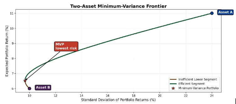
Figure 2 shows a two-asset minimum-variance frontier. The star marks the minimum-variance portfolio, which has the lowest standard deviation on the curve. The segment above the minimum-variance portfolio is efficient because moving upward on that segment increases expected return as risk rises. The lower segment is inefficient because, for the same risk, a portfolio on the upper segment offers a higher expected return.

Two-Asset Portfolio Variance

For a two-asset portfolio, portfolio variance is:

$$
\sigma_P^2 = w_A^2 \sigma_A^2 + w_B^2 \sigma_B^2 + 2 w_A w_B \sigma_{A,B}
$$

Where:

• \( \sigma_P^2 \) is the portfolio variance<
• \( w_A \) is the weight of Asset A
• \( w_B \) is the weight of Asset B
• \( \sigma_A^2 \) is the variance of returns for Asset A
• \( \sigma_B^2 \) is the variance of returns for Asset B
• \( \sigma_{A,B} \)= is the covariance between the returns of Assets A and B

When correlation is given instead of covariance, covariance is calculated as:

$$
\sigma_{A,B} = \rho_{A,B} \sigma_A \sigma_B
$$

Where:

• \( \sigma_{A,B} \) is the covariance between returns on Assets A and B
• \( \rho_{A,B} \) is the correlation between returns on Assets A and B
• \( \sigma_A \) is the standard deviation of returns on Asset A
• \( \sigma_B \) is the standard deviation of returns on Asset B

Covariance is the term that creates diversification. When covariance is low or negative, the portfolio can achieve a lower risk than a simple weighted average of the individual asset risks. When covariance is high, diversification benefits are weaker.

Minimum-Variance Weights for Two Assets

For a two-asset portfolio, the weight of Asset A in the minimum-variance portfolio is:

$$
w_{A,min} = \frac{\sigma_B^2 – \sigma_{A,B}}{\sigma_A^2 + \sigma_B^2 – 2\sigma_{A,B}}
$$

Where:

• \( w_{A,min} \) is the minimum-variance weight of Asset A
• \( \sigma_B^2 \) is the variance of returns for Asset B
• \( \sigma_A^2 \) is the variance of returns for Asset A
• \( \sigma_{A,B} \) is the covariance between the returns of Assets A and B

The weight of Asset B is:

$$
w_{B,min} = 1 – w_{A,min}
$$

Where:

• \( w_{B,min} \) is the minimum-variance weight of Asset B
• \( w_{A,min} \) is the minimum-variance weight of Asset A

The formula minimizes variance only. Expected returns are not used in the calculation of the minimum-variance weights. Expected returns matter later when identifying which portfolios lie on the efficient segment of the frontier and when matching portfolios to investor preferences.

Example 1: Calculating the Minimum-Variance Portfolio

Assume we have two investable funds. Asset A is a clean-energy equity fund with an expected return of 11.0% and a standard deviation of 24.0%. Asset B is an infrastructure credit fund with an expected return of 6.0% and a standard deviation of 10.0%. The estimated correlation between the two funds is 0.15. Calculate the minimum-variance weights and interpret the result.

Solution

Start by quoting the covariance formula:

$$
\sigma_{A,B} = \rho_{A,B} \sigma_A \sigma_B
$$

Where:

• \( \rho_{A,B} = 0.15 \) is the correlation between Asset A and Asset B
• \( \sigma_A = 24.0\% = 0.240 \) is the standard deviation of Asset A
• \( \sigma_B = 10.0\% = 0.100 \) is the standard deviation of Asset B
• \( \sigma_{A,B} \) is the covariance between the two asset returns

Calculate covariance:

$$
\sigma_{A,B} = 0.15(0.240)(0.100) = 0.0036
$$

Now quote the minimum-variance weight formula:

$$
w_{A,min} = \frac{\sigma_B^2 – \sigma_{A,B}}{\sigma_A^2 + \sigma_B^2 – 2\sigma_{A,B}}
$$

Where:

• \( w_{A,min} \) is the minimum-variance weight of Asset A
• \( \sigma_A^2 = (0.240)^2 = 0.0576 \) is the variance of Asset A
• \( \sigma_B^2 = (0.100)^2 = 0.0100 \) is the variance of Asset B
• \( \sigma_{A,B} = 0.0036 \) is the covariance between Asset A and Asset B

Substitute the values:

$$
w_{A,min} = \frac{0.0100 – 0.0036}{0.0576 + 0.0100 – 2(0.0036)} = 0.1060
$$

The weight of Asset B is:

$$
w_{B,min} = 1 – 0.1060 = 0.8940
$$

The minimum-variance portfolio is therefore 10.60% in Asset A and 89.40% in Asset B.

To calculate the expected return, quote the formula:

$$
E(r_P) = w_A E(r_A) + w_B E(r_B)
$$

Where:

• \( E(r_P) \) is the expected return of the portfolio
• \( w_A = 10.60\% \) is the weight of Asset A
• \( w_B = 89.40\% \) is the weight of Asset B
• \( E(r_A) = 11.0\% \) is the expected return of Asset A
• \( E(r_B) = 6.0\% \) is the expected return of Asset B

Substitute the values:

$$
E(r_P) = 0.1060(11.0\%) + 0.8940(6.0\%) = 6.53\%
$$

To calculate the standard deviation, use the two-asset variance formula:

$$
\sigma_P^2 = w_A^2 \sigma_A^2 + w_B^2 \sigma_B^2 + 2w_A w_B \sigma_{A,B}
$$

Where:

• \( w_A = 0.1060 \) is the weight of Asset A
• \( w_B = 0.8940 \) is the weight of Asset B
• \( \sigma_A^2 = 0.0576 \) is the variance of Asset A
• \( \sigma_B^2 = 0.0100 \) is the variance of Asset B
• \( \sigma_{A,B} = 0.0036 \) is the covariance between the two asset returns

Substitute the values:

$$
\begin{align}
\sigma_P^2 &= (0.1060)^2(0.0576) + (0.8940)^2(0.0100) + 2(0.1060)(0.8940)(0.0036) \\
\sigma_P &= 9.65\%
\end{align}
$$

The minimum-variance portfolio has a relatively low allocation to the higher-volatility clean-energy equity fund. This is not because the equity fund has a lower expected return; it does not. The reason is that the calculation is minimizing variance, so the lower-volatility infrastructure credit fund receives most of the weight.

The Minimum-Variance Frontier Versus the Efficient Frontier

The minimum-variance frontier contains the lowest-risk portfolios for different levels of expected return. The efficient frontier is the upper part of that frontier, beginning at the global minimum-variance portfolio and moving upward toward portfolios with higher expected returns and higher standard deviations.

The distinction matters because the lower part of the minimum-variance frontier is dominated. A portfolio on the lower branch has the same risk as another portfolio on the upper branch but a lower expected return. A risk-averse investor would not choose the lower-branch portfolio under mean-variance preferences.

$$ \textbf{Table 2: Minimum-Variance Frontier and Efficient Frontier} \\
\begin{array}{l|l|l}
\textbf{Concept} & \textbf{Meaning} & \textbf{Key Interpretation} \\
\hline
\text{Minimum-variance frontier} & \text{Set of portfolios with the lowest} & \text{Contains both efficient and} \\
& \text{variance for different expected} & \text{inefficient segments} \\
& \text{return levels} & \\
\hline
\text{Efficient frontier} & \text{Upper segment of the} & \text{Contains portfolios that are not} \\
& \text{minimum-variance frontier} & \text{dominated} \\
\hline
\text{Global minimum-variance portfolio} & \text{Lowest-risk portfolio on the frontier} & \text{Starting point of the efficient} \\
& & \text{frontier} \\
\hline
\text{Lower branch} & \text{Portfolios below the global} & \text{Inefficient because higher-return} \\
& \text{minimum-variance portfolio} & \text{alternatives exist at similar risk}
\end{array}
$$

Table 2 is one of the most important conceptual distinctions in this learning outcome. The efficient frontier is not the entire curve; it is the portion of the curve that investors would consider after eliminating dominated portfolios.

Target Return and Frontier Weights

For two assets, once the target portfolio return is specified, the asset weights can be determined from the expected return constraint:

$$
r_P = w_A r_A + w_B r_B
$$

Where:

• \( r_P \) is the target expected return of the portfolio
• \( w_A \) is the weight of Asset A
• \( w_B \) is the weight of Asset B
• \( r_A \) is the expected return of Asset A
• \( r_B \) is the expected return of Asset B

Because the weights must sum to one, the weight of Asset A can be written as:

$$
w_A = \frac{r_P – r_B}{r_A – r_B}
$$

Where:

• \( w_A \) is the weight of Asset A needed to reach target return \( r_P \)
• \( r_P \) is the target expected return of the portfolio
• \( r_A \) is the expected return of Asset A
• \( r_B \) is the expected return of Asset B

The weight of Asset B is:

$$
w_B = \frac{r_A – r_P}{r_A – r_B}
$$

Where:

• \( w_B \) is the weight of Asset B needed to reach target return \( r_P \)
• \( r_A \) is the expected return of Asset A
• \(r_B\) is the expected return of Asset B
• \(r_P\) is the target expected return of the portfolio

If short selling is not permitted, the target return must be feasible with non-negative weights. With only two long-only assets, the target expected return must lie between the expected returns of the two assets.

Example 2: Locating a Portfolio on the Efficient Frontier

Let us continue with the clean-energy equity fund and infrastructure credit fund from Example 1. A client has a target expected return of 8.0%. The analyst wants to know which asset weights would achieve that target and whether the portfolio lies on the efficient segment of the frontier.

Solution

The target-return weight formula is given by:

$$
w_A = \frac{r_P – r_B}{r_A – r_B}
$$

Where:

• \( w_A \) is the weight of Asset A
• \( r_P = 8.0\% \) is the target expected return
• \( r_A = 11.0\% \) is the expected return of Asset A
• \( r_B = 6.0\% \) is the expected return of Asset B

Substitute the values:

$$
w_A = \frac{8.0\% – 6.0\%}{11.0\% – 6.0\%} = 40.0\%
$$

The weight of Asset B is:

$$
w_B = 1 – 40.0\% = 60.0\%
$$

Next, calculate the portfolio variance using:

$$
\sigma_P^2 = w_A^2 \sigma_A^2 + w_B^2 \sigma_B^2 + 2w_A w_B \sigma_{A,B}
$$

Where:

• \( w_A = 0.400 \) is the weight of Asset A
• \( w_B = 0.600 \) is the weight of Asset B
• \( \sigma_A^2 = 0.0576 \) is the variance of Asset A
• \( \sigma_B^2 = 0.0100 \) is the variance of Asset B
• \( \sigma_{A,B} = 0.0036 \) is the covariance between Asset A and Asset B

Substitute the values:

$$
\begin{align}
\sigma_P^2 &= (0.400)^2(0.0576) + (0.600)^2(0.0100) + 2(0.400)(0.600)(0.0036) = 0.014544 \\
\sigma_P &= \sqrt{0.014544} = 12.06\%
\end{align}
$$

The target-return portfolio is 40.0% in Asset A and 60.0% in Asset B, with a standard deviation of 12.06%. Because its expected return of \( 8.0\% \) is above the minimum-variance portfolio return of \( 6.53\% \), it lies on the efficient segment of the two-asset frontier.

Interpreting Portfolios on the Efficient Frontier

Portfolios on the efficient frontier are not all equally suitable for a specific investor. A more conservative investor may prefer a portfolio near the lower-left part of the efficient frontier, close to the global minimum-variance portfolio. An investor willing to bear greater risk for higher expected return may prefer a portfolio farther up and to the right.

The key idea is dominance. A portfolio is dominated if another available portfolio offers higher expected return for the same risk or lower risk for the same expected return. Efficient portfolios are not dominated. Inefficient portfolios are dominated and should generally be rejected in a mean-variance framework.

Figure 3: Three Ways to Frame Portfolio Optimization

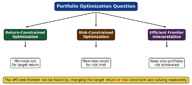
Figure 3 organizes the main optimization approaches. A return-constrained problem asks for the lowest-risk portfolio that reaches a target return. A risk-constrained problem asks for the highest expected return that can be achieved without exceeding a risk limit. Efficient-frontier interpretation then eliminates dominated portfolios and leaves the set of candidate portfolios for investor choice.

Optimization with more than Two Assets

With more than two assets, the intuition is the same but the calculation becomes more demanding. Expected returns, standard deviations, and covariances must be estimated for all assets. A covariance matrix then allows the analyst to calculate portfolio variance for many combinations of weights.

The matrix form of portfolio variance is:

$$
\sigma_P^2 = w^T V w
$$

Where:

• \( \sigma_P^2 \) is the portfolio variance
• \( w \) is the column vector of portfolio weights
• \( w^T \) is the transpose of the weight vector
• \( V \) is the covariance matrix of asset returns

This notation is compact, but the investment logic remains familiar. The optimizer searches across possible weights and identifies portfolios that satisfy the constraints while improving the risk-return trade-off.

$$ \textbf{Table 3: Key Inputs in Mean-Variance Optimization} \\
\begin{array}{l|l|l}
\textbf{Input} & \textbf{Role in the Optimization} & \textbf{Common Practical Challenge} \\
\hline
\text{Expected returns} & \text{Determine which portfolios offer} & \text{Forecasts can be unstable and} \\
& \text{higher anticipated reward} & \text{model dependent} \\
\hline
\text{Standard deviations} & \text{Measure standalone asset risk} & \text{Historical volatility may not reflect} \\
& & \text{future regimes} \\
\hline
\text{Covariances or correlations} & \text{Capture diversification effects} & \text{Correlations may rise during} \\
& & \text{market stress} \\
\hline
\text{Portfolio constraints} & \text{Translate investment policy into} & \text{Constraints can narrow or reshape} \\
& \text{feasible weights} & \text{the efficient frontier} \\
\hline
\text{Target return or risk limit} & \text{Defines the optimization question} & \text{Targets may be unrealistic relative} \\
& & \text{to the available assets}
\end{array}
$$

Table 3 also explains why optimization output should not be accepted blindly. Efficient frontiers can be highly sensitive to inputs. Small changes in expected returns or correlations may materially change recommended portfolio weights.

Example 3: Comparing Return-Constrained and Risk-Constrained Optimization

Imagine a multi-asset analyst is evaluating three broad allocations: a global equity fund, a sustainable credit fund, and a short-term government securities fund. The analyst is not asked to solve a full numerical optimizer by hand. Instead, the task is to interpret two optimization outputs produced by portfolio software.

$$ \begin{array}{l|c|c}
\textbf{Asset} & \textbf{Return-Constrained} & \textbf{Risk-Constrained} \\
& \textbf{Portfolio} & \textbf{Portfolio} \\
\hline
\text{Global Equity Fund} & 46.0\% & 34.0\% \\ \hline
\text{Sustainable Credit Fund} & 38.0\% & 41.0\% \\ \hline
\text{Short-Term Government Securities} & 16.0\% & 25.0\% \\ \hline
\text{Expected Portfolio Return} & 9.50\% & 8.20\% \\ \hline
\text{Expected Portfolio Standard Deviation} & 11.90\% & 9.00\%
\end{array}
$$

The return-constrained portfolio was built to achieve at least 9.50% expected return while minimizing risk. The risk-constrained portfolio was built to keep expected standard deviation at 9.00% while maximizing expected return.
The interpretation is direct. The return-constrained portfolio has a larger global equity allocation because the return target is higher. The risk-constrained portfolio has a larger allocation to short-term government securities because the volatility limit is tighter. Both portfolios may lie on the efficient frontier, but they answer different portfolio construction questions.

This example also shows why the phrase “optimal portfolio” must be handled carefully. A portfolio can be optimal for a return target, optimal for a risk limit, or optimal for a risk-adjusted objective. It is not meaningful to call a portfolio optimal without specifying the investor’s objective and constraints.

Common Interpretation Traps

A few traps appear frequently in exam questions.

First, the minimum-variance portfolio is not necessarily the highest-return portfolio. It is the lowest-risk feasible portfolio. Second, the efficient frontier is not the full feasible set. It is the upper boundary of the feasible set after dominated portfolios have been removed. Third, the lower branch of the minimum-variance frontier is not efficient because portfolios on the upper branch offer higher expected return at the same risk. Fourth, expected return is not used in the two-asset minimum-variance weight formula, but it is essential when identifying portfolios for a target return or interpreting the efficient frontier.

Finally, constraints matter. A no-short-sale constraint can force the solution to a boundary. For example, if the unconstrained minimum-variance formula gives a negative weight for an asset, a long-only investor cannot use that weight. The constrained minimum-variance portfolio may then place zero weight in that asset.

Interpretation and Evaluation

Several practical principles follow:

• The feasible set contains all portfolios allowed by the available assets and constraints.
• The efficient frontier contains only the non-dominated portfolios.
• The global minimum-variance portfolio has the lowest variance among all feasible portfolios.
• The efficient frontier begins at the global minimum-variance portfolio and extends upward toward higher-risk, higher-return portfolios.
• The lower branch of the minimum-variance frontier is inefficient.
• Minimum-variance weights depend on variances and covariance, not expected returns.
• Target-return portfolio weights depend on expected returns and the target return.
• Optimization output depends heavily on input estimates and constraints.

Question

Asset A has an expected return of 9.0% and a standard deviation of 12.0%. Asset B has an expected return of 14.0% and a standard deviation of 22.0%. The correlation between the two asset returns is 0.25.

The weight of Asset A in the two-asset minimum-variance portfolio is closest to:

1. 15.7%
2. 77.1%
3. 84.3%

Answer Explanation

The correct answer is C.

Start by quoting the covariance formula:

$$
\sigma_{A,B} = \rho_{A,B} \sigma_A \sigma_B
$$

Where:

• \( \sigma_{A,B} \) is the covariance between returns on Asset A and Asset B
• \( \rho_{A,B} = 0.25 \) is the correlation between the two asset returns
• \( \sigma_A = 12.0\% = 0.120 \) is the standard deviation of Asset A
• \( \sigma_B = 22.0\% = 0.220 \) is the standard deviation of Asset B

Calculate covariance:

$$
\sigma_{A,B} = 0.25(0.120)(0.220) = 0.0066
$$

Now the minimum-variance weight formula is given by:

$$
w_{A,min} = \frac{\sigma_B^2 – \sigma_{A,B}}{\sigma_A^2 + \sigma_B^2 – 2\sigma_{A,B}}
$$

Where:

• \( w_{A,min} \) is the minimum-variance weight of Asset A
• \( \sigma_A^2 = (0.120)^2 = 0.0144 \) is the variance of Asset A
• \( \sigma_B^2 = (0.220)^2 = 0.0484 \) is the variance of Asset B
• \( \sigma_{A,B} = 0.0066 \) is the covariance between the two asset returns

Substitute the values:

$$
w_{A,min} = \frac{0.0484 – 0.0066}{0.0144 + 0.0484 – 2(0.0066)} = \frac{0.0418}{0.0496} = 0.8427
$$

The weight of Asset A in the minimum-variance portfolio is approximately 84.3%.

A is incorrect because 15.7% is the weight of Asset B, calculated as \( 1 – 0.8427 \).

B is incorrect because 77.1% is obtained by ignoring covariance and using \(\frac {0.0484}{(0.0144 + 0.0484)} \).