Hypothesis Testing in Finance: Significance, Type I and Type II Errors

Why Hypothesis Testing Matters

Investment professionals frequently need to decide whether an observed result is meaningful or merely the product of sampling variation. A fund may outperform its benchmark over three years. A new systematic strategy may show higher average returns than an existing strategy. A risk model may appear to underestimate volatility. In each case, the analyst is asking the same practical question: is the sample evidence strong enough to support a conclusion about the underlying population?

Hypothesis testing is the statistical framework used to answer that question. It begins with a claim about a population parameter and then evaluates whether the sample evidence is consistent with that claim. The conclusion is always framed in relation to the null hypothesis: the analyst either rejects the null hypothesis or fails to reject it. The analyst does not prove the null hypothesis true.

In investment practice, hypothesis testing is used to evaluate return expectations, risk estimates, manager performance, correlations, and strategy claims. It is especially important when a result is economically interesting but statistically uncertain. A small performance difference may look attractive in a presentation, but a hypothesis test helps determine whether the difference is large relative to the noise in the data.

Parametric and Non-Parametric Testing Context

Hypothesis tests may be parametric or non-parametric. A parametric test relies on assumptions about the distribution of the data or the parameter being tested. For example, a t-test for a mean assumes that the relevant statistic follows a t-distribution under the null hypothesis. A chi-square test for variance and an F-test for comparing variances are also parametric tests.

A non-parametric test does not require the same distributional assumptions. It may be more appropriate when the data are ordinal, highly non-normal, or contain severe outliers. This learning outcome focuses on the core hypothesis testing framework and the main parametric tests. Non-parametric tests are treated more fully in the next learning outcome.

The Hypothesis Testing Process

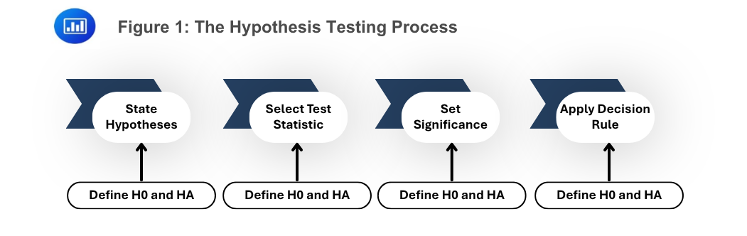
Figure 1 summarizes the logic of hypothesis testing. First, state the null and alternative hypotheses. Second, identify the test statistic and its distribution. Third, specify the level of significance. Fourth, compare the test statistic with the decision rule and interpret the result. This four-step structure should be visible in any well-written solution.

The process can be summarized as follows:

1. State the null and alternative hypotheses
2. Identify the test statistic and its distribution
3. Specify the level of significance
4. Establish the decision rule and interpret the result

The order matters. A test should not begin with a desirable answer and then search for a statistic that supports it. The hypotheses, significance level, and decision rule should be set before the sample evidence is interpreted.

Null and Alternative Hypotheses

The null hypothesis, written as H₀, is the statement initially assumed to hold unless the sample evidence is strong enough to reject it. The null often represents no effect, no difference, no improvement, or a benchmark condition.

The alternative hypothesis, written as H_a, is the statement supported if the null is rejected. The alternative usually reflects the effect, difference, improvement, deterioration, or relationship that the analyst is trying to establish.

The null and alternative hypotheses must be mutually exclusive and collectively exhaustive. They cannot overlap, and together they must cover all possible values of the parameter.

A useful rule is that the equality sign belongs in the null hypothesis. The null can be stated using =, \(\leq\), or \(\geq\). The alternative is usually stated using \(\neq\), \(\gt\), or \(\lt\), depending on the research question.

$$ \textbf{Table 1: General Forms of Hypothesis Tests} \\
\begin{array}{l|c|c|c}
\textbf{Test Type} & \textbf{Null Hypothesis} & \textbf{Alternative Hypothesis} & \textbf{Rejection Region} \\
\hline
\text{Right-tail test} & H_0: \theta \leq \theta_0 & H_a: \theta > \theta_0 & \text{Right tail} \\
\text{Left-tail test} & H_0: \theta \geq \theta_0 & H_a: \theta < \theta_0 & \text{Left tail} \\ \text{Two-tailed test} & H_0: \theta = \theta_0 & H_a: \theta \neq \theta_0 & \text{Both tails} \end{array} $$

Table 1 is central. If the analyst wants to test whether a new strategy produces returns greater than zero, the alternative is right-tailed. If the analyst wants to test whether tracking error is lower than a limit, the alternative is left-tailed. If the analyst wants to test whether a parameter is different from a benchmark in either direction, the alternative is two-tailed.

Example 1: Formulating a Right-Tail Hypothesis Test

Suppose we want to test whether a new machine-learning equity strategy produces positive mean monthly alpha after transaction costs. The parameter of interest is the population mean monthly alpha, \( \mu \). The benchmark value is zero.

The analyst’s claim is that the strategy produces alpha greater than zero. This claim should be placed in the alternative hypothesis. The hypotheses are:

$$
\begin{array}{l}
H_0: \mu \leq 0 \\
H_a: \mu > 0
\end{array}
$$

Where:

• \( H_0 \) is the null hypothesis
• \( H_a \) is the alternative hypothesis
• \( \mu \) is the population mean monthly alpha
• 0 is the benchmark alpha level

This is a right-tail test because evidence against the null occurs when the sample mean alpha is sufficiently high. The test is not formulated as \( H_0: \mu > 0 \) because the claim of positive alpha should not be assumed true without sample evidence.

One-Tailed and Two-Tailed Tests

Figure 2: Rejection Regions for One-Tailed and Two-Tailed Tests

Figure 2 shows how the alternative hypothesis determines the rejection region. A right-tail test looks for unusually large positive values. A left-tail test looks for unusually large negative values. A two-tailed test looks for unusually large deviations in either direction. For the same significance level, a two-tailed test splits the rejection probability across two tails.

The choice between one-tailed and two-tailed testing must be driven by the research question. If only outperformance matters, a right-tail test may be justified. If underperformance and outperformance both matter, a two-tailed test is more appropriate.

Test Statistics and their Distributions

A test statistic converts sample evidence into a standardized number that can be compared with a probability distribution under the null hypothesis. The correct test statistic depends on the population parameter being tested, the sample structure, and the assumptions of the test.

Figure 3: Choosing the Test Statistic

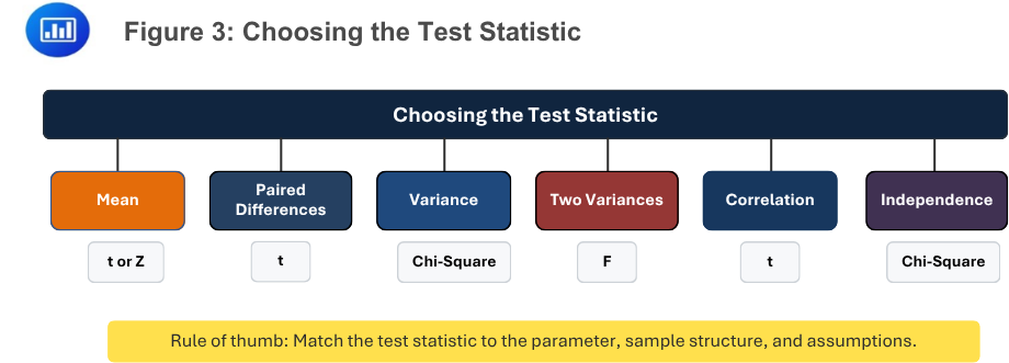
Figure 3 provides a practical map. Tests of means usually use a t-statistic when the population variance is unknown. Tests of a single variance use a chi-square statistic. Tests comparing two variances use an F-statistic. Tests of correlation use a t-statistic based on the sample correlation and sample size.

$$ \textbf{Table 2: Common Parametric Tests} \\
\begin{array}{l|l|l|l}
\textbf{What is being Tested?} & \textbf{Common Test Statistic} & \textbf{Distribution under the Null} & \textbf{Typical Degrees of Freedom} \\
\hline
\text{Single mean} & \text{t-statistic} & \text{t-distribution} & n-1 \\ \hline
\text{Single variance} & \text{Chi-square statistic} & \text{Chi-square distribution} & n-1 \\ \hline
\text{Difference in two means} & \text{t-statistic} & \text{t-distribution} & \text{Depends on test assumptions} \\ \hline
\text{Difference in two variances} & \text{F-statistic} & \text{F-distribution} & n_1-1, n_2-1 \\ \hline
\text{Paired differences} & \text{t-statistic} & \text{t-distribution} & n-1 \\ \hline
\text{Correlation} & \text{t-statistic} & \text{t-distribution} & n-2
\end{array}
$$

Table 2 should not be memorized mechanically. The test statistic follows from the parameter and the sample structure. Testing a mean is different from testing a variance. Comparing independent samples is different from evaluating paired observations. Testing a correlation is different from comparing means.

Testing a Single Mean

For a hypothesis test involving a single population mean, the t-statistic is commonly used when the population standard deviation is unknown:

$$
t = \frac{\bar{X}-\mu_0}{s/\sqrt{n}}
$$

Where:

• \( t \) is the test statistic
• \( \bar{X} \) is the sample mean
• \( \mu_0 \) is the hypothesized population mean under \( H_0 \)
• \( s \) is the sample standard deviation
• \( n \) is the sample size

The statistic measures how many estimated standard errors the sample mean is away from the hypothesized value. A larger absolute t-statistic means the sample mean is farther from the null value after adjusting for sample variability.

Example 2: Testing whether Mean Alpha is Positive

Suppose we want to test whether an equity long-short strategy has positive mean monthly alpha. The analyst observes 64 monthly alphas. The sample mean is \( 0.72\% \), and the sample standard deviation is \( 3.20\% \). The test is conducted at the \( 5\% \) level of significance using a right-tail test. The critical t-value is 1.669.

Solution

We know that:

$$
t = \frac{\bar{X}-\mu_0}{s/\sqrt{n}}
$$

Where:

• \( \bar{X}=0.72\% \) is the sample mean monthly alpha
• \( \mu_0=0\% \) is the hypothesized alpha under the null hypothesis
• \( s=3.20\% \) is the sample standard deviation of monthly alpha
• \( n=64 \) is the number of monthly observations
• \( t \) is the test statistic

The hypotheses are:

$$
\begin{array}{l}
H_0: \mu \leq 0 \\
H_a: \mu > 0
\end{array}
$$

Calculate the test statistic:

$$
t = \frac{0.72\%-0\%}{3.20\%/\sqrt{64}} = 1.80
$$

Because \( 1.80 > 1.669 \), the test statistic falls in the right-tail rejection region. The analyst rejects \( H_0 \) at the \( 5\% \) level and concludes that the sample provides statistically significant evidence of positive mean monthly alpha.

The conclusion is statistical, not a guarantee of future performance. Transaction costs, crowding, model decay, capacity, and market regime changes could still undermine the strategy going forward.

Testing a Single Variance

A test of a single population variance uses the chi-square statistic:

$$
\chi^2 = \frac{(n-1)s^2}{\sigma_0^2}
$$

Where:

• \( \chi^2 \) is the chi-square test statistic
• \( n \) is the sample size
• \( s^2 \) is the sample variance
• \( \sigma_0^2 \) is the hypothesized population variance

The statistic follows a chi-square distribution with \( n-1 \) degrees of freedom when the population is normally distributed. Variance tests are useful in risk management when the analyst wants to test whether volatility is above or below a policy threshold, model assumption, or benchmark level.

Example 3: Testing whether Variance Exceeds a Risk Limit

A commodity strategy has been evaluated using 30 monthly returns. The sample variance of returns is 0.0064, while the risk committee’s variance threshold is 0.0049. Conduct a right‑tailed chi‑square test at the 5% significance level to determine whether the return variance exceeds the threshold. The critical chi‑square value with 29 degrees of freedom is 42.557.

Solution

We know that:

$$
\chi^2 = \frac{(n-1)s^2}{\sigma_0^2}
$$

Where:

• \( n=30 \) is the number of monthly return observations
• \( s^2=0.0064 \) is the sample variance
• \( \sigma_0^2=0.0049 \) is the hypothesized variance threshold
• \( \chi^2 \) is the chi-square test statistic

The hypotheses are:

$$
\begin{array}{l}
H_0: \sigma^2 \leq 0.0049 \\
H_a: \sigma^2 > 0.0049
\end{array}
$$

Calculate the test statistic:

$$
\chi^2 = \frac{(30-1)(0.0064)}{0.0049} = 37.88
$$

Because \( 37.88 < 42.557 \), the analyst fails to reject \( H_0 \). The sample variance is higher than the threshold numerically, but it is not high enough relative to sampling uncertainty to conclude statistical significance at the \( 5\% \) level.

Testing the Difference between Two Means

Many investment questions compare two return streams. An analyst may ask whether a growth strategy has higher average returns than a value strategy, whether a new model outperforms the legacy model, or whether post-event returns differ from pre-event returns.

For two independent samples, a common t-statistic is:

$$
t = \frac{(\bar{X}_1-\bar{X}_2)-\Delta_0}{\sqrt{s_1^2/n_1+s_2^2/n_2}}
$$

Where:

• \( t \) is the test statistic for the difference in means
• \( \bar{X}_1 \) is the sample mean of group 1
• \( \bar{X}_2 \) is the sample mean of group 2
• \( \Delta_0 \) is the hypothesized difference between the population means
• \( s_1^2 \) is the sample variance of group 1
• \( s_2^2 \) is the sample variance of group 2
• \( n_1 \) is the sample size of group 1
• \( n_2 \) is the sample size of group 2

If the samples are independent and the two population variances are assumed equal, the analyst may use a pooled-variance version of the test. If the samples are paired, the analyst should usually use a paired-difference test instead of treating the two samples as independent.

Example 4: Testing the Difference between Two Independent Strategy Means

Assume an analyst wants to test whether a low-volatility equity strategy earned a different average monthly return from a quality equity strategy. The analyst uses 48 monthly returns for each strategy. The low-volatility strategy has a mean monthly return of \( 0.95\% \) and a variance of \( 0.0016 \). The quality strategy has a mean monthly return of \( 0.60\% \) and a variance of \( 0.0012 \). The test is two-tailed, and the hypothesized mean difference is zero. The \( 5\% \) critical t-values are approximately \( \pm1.986 \).

Solution

Recall that:

$$
t = \frac{(\bar{X}_1-\bar{X}_2)-\Delta_0}{\sqrt{s_1^2/n_1+s_2^2/n_2}}
$$

Where:

• \( \bar{X}_1=0.95\% \) is the mean return of the low-volatility strategy
• \( \bar{X}_2=0.60\% \) is the mean return of the quality strategy
• \( \Delta_0=0\% \) is the hypothesized difference in mean returns
• \( s_1^2=0.0016 \) is the variance of the low-volatility strategy
• \( s_2^2=0.0012 \) is the variance of the quality strategy
• \( n_1=48 \) and \( n_2=48 \) are the sample sizes

The hypotheses are:

$$
\begin{array}{l}
H_0: \mu_1 – \mu_2 = 0 \\
H_a: \mu_1 – \mu_2 \neq 0
\end{array}
$$

Calculate the test statistic using decimal returns:

$$
t = \frac{0.0095-0.0060-0}{\sqrt{\frac{0.0016}{48}+\frac{0.0012}{48}}} = 0.46
$$

Because \( |0.46| < 1.986 \), the analyst fails to reject \( H_0 \). The two sample means differ numerically, but the evidence is insufficient to conclude that the population mean returns are statistically different at the \( 5\% \) level.

Testing the Difference Between Two Variances

To compare two population variances, the F-statistic is commonly used:

$$
F = \frac{s_1^2}{s_2^2}
$$

Where:

• \( F \) is the F-test statistic
• \( s_1^2 \) is the sample variance of the first population
• \( s_2^2 \) is the sample variance of the second population

The F-statistic follows an F-distribution with \( n_1-1 \) and \( n_2-1 \) degrees of freedom under the null hypothesis when both populations are normally distributed. In practice, the sample with the larger variance is often placed in the numerator when the test is formulated to identify whether one variance exceeds another.

Example 5: Testing Whether One Volatility Is Greater Than Another

The goal is to test whether the monthly return variance of a thematic technology fund is greater than that of a diversified equity index. The technology fund has a sample variance of 0.0049 based on 36 months, while the diversified index has a sample variance of 0.0025 based on 36 months. The right-tail F-test is conducted at the \( 5\% \) level, and the critical F-value is 1.76.

Solution

F-statistic is given by:

$$
F = \frac{s_1^2}{s_2^2}
$$

Where:

• \( s_1^2=0.0049 \) is the sample variance of the thematic technology fund
• \( s_2^2=0.0025 \) is the sample variance of the diversified equity index
• \( F \) is the F-test statistic

The hypotheses are:

$$
\begin{array}{l}
H_0: \sigma_1^2 \leq \sigma_2^2 \\
H_a: \sigma_1^2 > \sigma_2^2
\end{array}
$$

Calculate the F-statistic:

$$
F = \frac{0.0049}{0.0025} = 1.96
$$

Because \( 1.96 > 1.76 \), the analyst rejects \( H_0 \) at the \( 5\% \) level. The sample provides statistically significant evidence that the thematic technology fund has higher variance than the diversified equity index.

Testing Paired Differences

A paired-difference test is used when observations naturally belong together. Examples include before-and-after returns for the same securities, matched portfolio returns under two weighting rules, or monthly returns between a fund and its benchmark. The test works by creating a new series of paired differences and then testing the mean of those differences.

The t-statistic for paired differences is:

$$
t = \frac{\bar{d}-\mu_0}{s_d/\sqrt{n}}
$$

Where:

• \( t \) is the paired-difference test statistic
• \( \bar{d} \) is the mean of the paired differences
• \( \mu_0 \) is the hypothesized mean difference
• \( s_d \) is the sample standard deviation of the paired differences
• \( n \) is the number of paired observations

The key distinction is that a paired test uses the differences within each pair. This can improve power by controlling for factors that affect both observations in a pair.

Example 6: Testing a Mean Paired Difference

An analyst wants to test whether a portfolio’s monthly return differs from its benchmark after controlling for month-by-month market conditions. The analyst forms 36 paired differences by subtracting the benchmark return from the portfolio return each month. The mean monthly difference is \( 0.45\% \), and the sample standard deviation of the differences is \( 1.50\% \). The test is two-tailed at the \( 5\% \) level, and the critical values are \( \pm2.030 \).

Solution

We apply the formula:

$$
t = \frac{\bar{d}-\mu_0}{s_d/\sqrt{n}}
$$

Where:

• \( \bar{d}=0.45\% \) is the mean monthly portfolio-minus-benchmark difference
• \( \mu_0=0\% \) is the hypothesized mean difference
• \( s_d=1.50\% \) is the standard deviation of the paired differences
• \( n=36 \) is the number of paired monthly observations
• \( t \) is the paired-difference test statistic

The hypotheses are:

$$
\begin{array}{l}
H_0: \mu_d = 0 \\
H_a: \mu_d \neq 0
\end{array}
$$

Calculate the test statistic:

$$
t = \frac{0.45\%-0\%}{\frac {1.50\%}{\sqrt{36}}} = 1.80
$$

Because \( |1.80| < 2.030 \), the analyst fails to reject \( H_0 \). The portfolio outperformed the benchmark by \( 0.45\% \) per month in the sample, but the paired evidence is not statistically strong enough at the \( 5\% \) level.

Testing Correlation

A correlation test assesses whether the population correlation between two variables differs from a hypothesized value, most commonly zero. This is useful for testing whether two return series are meaningfully associated, whether a fund has exposure to a factor, or whether macroeconomic variables and asset returns are related.

The t-statistic for testing whether the population correlation is zero is:

$$
t = r \sqrt{\frac{n-2}{1-r^2}}
$$

Where:

• \( t \) is the test statistic for correlation
• \( r \) is the sample correlation coefficient
• \( n \) is the sample size

The statistic follows a t-distribution with \( n-2 \) degrees of freedom under the null hypothesis of zero correlation.

Example 7: Testing whether a Correlation is Significant

Assume we want to test whether monthly returns on a copper producer are statistically correlated with monthly copper price changes. The analyst observes 80 paired monthly observations and estimates a sample correlation of 0.28. The test is two-tailed at the \( 5\% \) level, and the critical values are approximately \( \pm1.991 \).

Solution

Recall the formula:

$$
t = r \sqrt{\frac{n-2}{1-r^2}}
$$

Where:

• \( r=0.28 \) is the sample correlation between the stock return and copper price change
• \( n=80 \) is the number of paired monthly observations
• \( t \) is the test statistic for the correlation test

The hypotheses are:

$$
\begin{array}{l}
H_0: \rho = 0 \\
H_a: \rho \neq 0
\end{array}
$$

Calculate the test statistic:

$$
t = 0.28 \sqrt{\frac{80-2}{1-0.28^2}} = 2.57
$$

Because \( |2.57| > 1.991 \), the analyst rejects \( H_0 \). The sample provides statistically significant evidence that the population correlation differs from zero. The conclusion should not be interpreted as proof that copper price changes cause the stock returns. It only supports a statistically significant linear association.

Significance Level, Critical Values, and Statistical Significance

The level of significance, \( \alpha \), is the probability of rejecting a true null hypothesis. It is the analyst’s tolerance for Type I error. Common values are \( 5\% \) and \( 1\% \).

The critical value is the boundary that separates the rejection region from the non-rejection region. Smaller values of \( \alpha \) require stronger evidence and therefore more extreme critical values.

A result is statistically significant if the test statistic falls in the rejection region or, equivalently, if the p-value is less than the chosen significance level. Statistical significance means the result is unlikely under the null hypothesis, given the assumptions of the test. It does not automatically mean the result is economically meaningful.

Type I Error, Type II Error, and Power of a Test

A Type I error occurs when a true null hypothesis is rejected. It is a false positive. The probability of a Type I error is \( \alpha \), the significance level.

A Type II error occurs when a false null hypothesis is not rejected. It is a false negative. The probability of a Type II error is \( \beta \).

The power of a test is the probability of correctly rejecting a false null hypothesis:

$$
Power = 1 – \beta
$$

Where:

• \( Power \) is the probability of correctly rejecting a false null hypothesis
• \( \beta \) is the probability of a Type I_I error

Figure 4: Type I Error, Type II Error, and Power

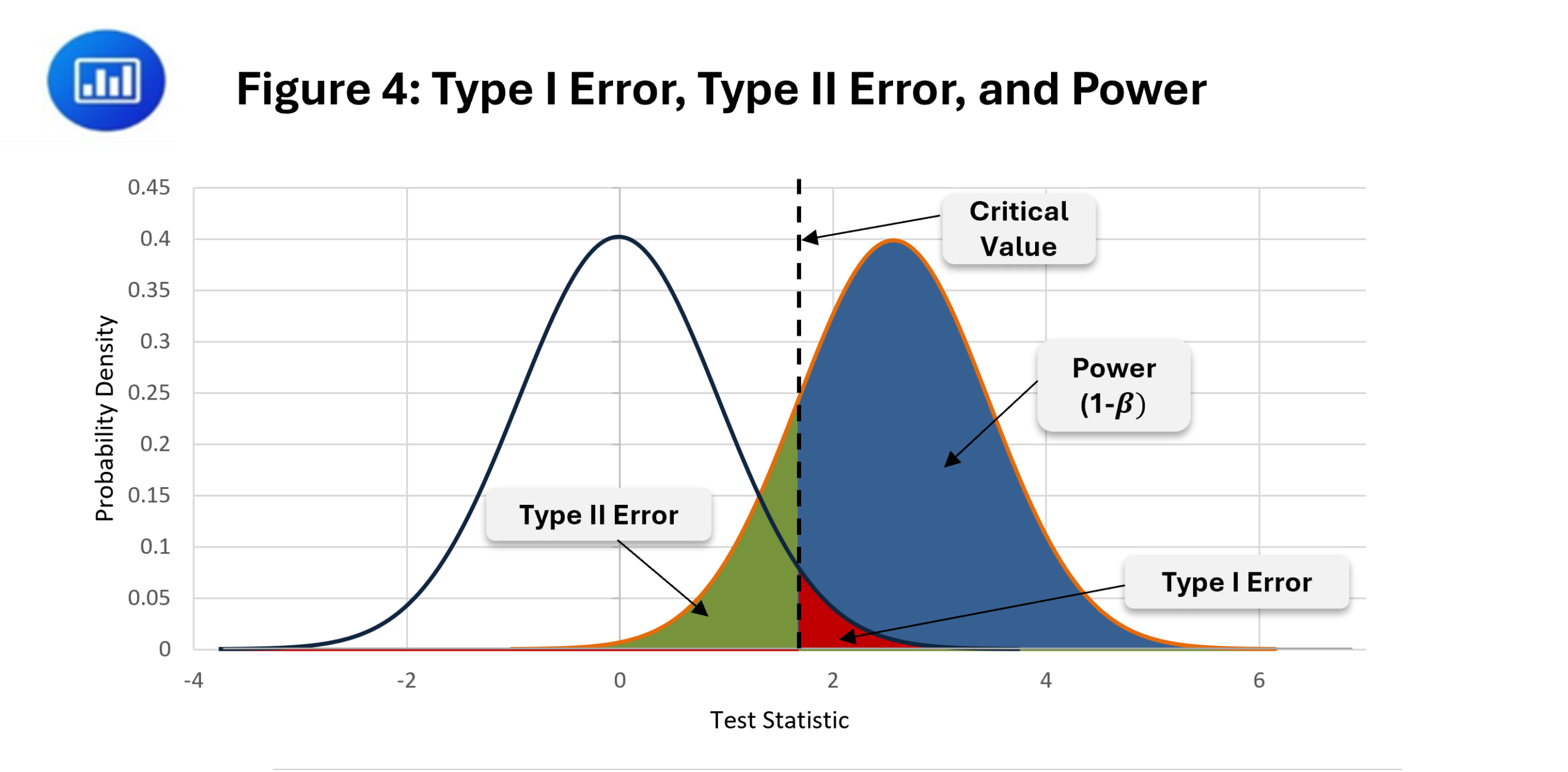
Figure 4 shows the trade-off. If the critical value is moved to make rejection easier, power rises, and Type II error falls, but the Type I error probability may increase. If the critical value is moved to make rejection harder, Type I error falls, but Type II error may rise. Increasing sample size can improve power without mechanically increasing \( \alpha \), which is why larger well-designed samples are valuable.

$$ \textbf{Table 3: Decisions and Errors in Hypothesis Testing} \\
\begin{array}{l|l|l}
\textbf{Decision} & \textbf{If } H_0 \textbf{ Is True} & \textbf{If } H_0 \textbf{ Is False} \\
\hline
\text{Fail to reject } H_0 & \text{Correct decision} & \text{Type II error, } \beta \\ \hline
\text{Reject } H_0 & \text{Type I error, } \alpha & \text{Correct decision; power, } 1-\beta
\end{array}
$$

Table 3 is one of the most important parts of the learning outcome. A Type I error can occur only when the null is rejected. A Type II error can occur only when the analyst fails to reject a false null.

The P-Value Approach

A p-value is the smallest significance level at which the null hypothesis would be rejected. It measures the probability, assuming the null is true, of observing a test statistic at least as extreme as the one obtained from the sample.

For a right-tail test:

$$
p = P(T \geq t_{obs} | H_0)
$$

Where:

• \( p \) is the p-value
• \( T \) is the test statistic under the null distribution
• \( t_{obs} \) is the observed test statistic
• \( H_0 \) is the null hypothesis

For a left-tail test:

$$
p = P(T \leq t_{obs} | H_0)
$$

Where:

• all terms are as previously defined

For a two-tailed test:

$$
p = 2P(T \geq |t_{obs}| | H_0)
$$

Where:

• \( |t_{obs}| \) is the absolute value of the observed test statistic
• all other terms are as previously defined

The decision rule is:

• Reject \( H_0 \) if \( p < \alpha \)
• Fail to reject \( H_0 \) if \( p \geq \alpha \)

The p-value approach and critical value approach lead to the same decision when applied correctly. The p-value also communicates strength of evidence. A p-value of 0.003 provides stronger evidence against \( H_0 \) than a p-value of 0.049, even though both are significant at the \( 5\% \) level.

P-Hacking and Ethical Interpretation

Hypothesis testing can be misused. P-hacking occurs when an analyst repeatedly changes the sample period, benchmark, variables, filters, or model specification until a statistically significant result appears. This practice increases the probability of Type I errors and can create misleading evidence for a strategy that does not truly work.

In investment management, p-hacking can appear as selective performance reporting, excessive data mining, benchmark switching, or removing unfavorable observations after seeing the results. The proper response is transparent methodology, economic reasoning, pre-specified tests where possible, out-of-sample validation, and honest reporting of unsuccessful tests.

Statistical significance should not be sold as investment truth. It should be treated as disciplined evidence under stated assumptions.

Interpretation and Evaluation

Several practical principles follow:

• The equality condition belongs in the null hypothesis.
• The alternative hypothesis determines whether the test is right-tailed, left-tailed, or two-tailed.
• The test statistic must match the parameter and sample structure.
• Statistical significance depends on the chosen significance level.
• A Type I error is rejecting a true null hypothesis.
• A Type II error is failing to reject a false null hypothesis.
• Power is the probability of correctly rejecting a false null hypothesis.
• Increasing sample size generally increases power and lowers the risk of Type II error.
• A statistically significant result may still be economically unimportant.
• P-hacking can turn ordinary noise into misleading evidence.

Question

An analyst tests whether a new intraday equity strategy generates positive mean daily alpha. The analyst observes 100 daily alpha observations, with a sample mean of \( 0.09\% \) and a sample standard deviation of \( 0.45\% \). The null and alternative hypotheses are:

$$
\begin{array}{l}
H_0: \mu \leq 0 \\
H_a: \mu > 0
\end{array}
$$

The test is conducted at the \( 5\% \) significance level, and the one-tailed critical t-value is 1.660. The analyst should most appropriately:

1. fail to reject H₀ because the calculated t-statistic is below the critical value
2. reject H₀ because the calculated t-statistic exceeds the critical value
3. reject H₀ because the p-value must be greater than the significance level

The correct answer is B.

Recall:

$$
t = \frac{\bar{X}-\mu_0}{s/\sqrt{n}}
$$

Where:

• \( t \) is the test statistic
• \( \bar{X}=0.09\% \) is the sample mean daily alpha
• \( \mu_0=0\% \) is the hypothesized mean daily alpha under the null hypothesis
• \( s=0.45\% \) is the sample standard deviation of daily alpha
• \( n=100 \) is the number of daily observations

Substitute the values:

$$
t = \frac{0.09\%-0\%}{\frac{0.45\%}{\sqrt{100}}} = 2.00
$$

Because \( 2.00 > 1.660 \), the calculated t-statistic falls in the right-tail rejection region. The analyst should reject \( H_0 \) at the \( 5\% \) significance level. The sample provides statistically significant evidence that the strategy’s mean daily alpha is positive.

A is incorrect because the calculated t-statistic, 2.00, is above the one-tailed critical value of 1.660.

C is incorrect because the p-value rule is the opposite: the analyst rejects \( H_0 \) when the p-value is less than the significance level, not greater than it.