Conditional Expectations, Variances, and Covariances in Financial Forecasting

From Unconditional Measures to Conditional Measures

The first learning outcome focused on unconditional mean, variance, and covariance. Those measures describe a random variable before any additional information is imposed. In investment practice, however, analysts rarely stop there. New information arrives constantly: inflation data are released, a central bank changes guidance, a company reports earnings, a credit rating changes, or a risk model identifies a new stress condition.

A conditional measure updates the analysis after some condition is known or assumed. The condition might be a market state, an economic scenario, a policy decision, or the realized value of another random variable. This is why conditional expectations are so useful in finance. They help the analyst move from a broad forecast to one specific to the information currently available.

For example, a portfolio’s unconditional expected return might be 6% for the next year. That number is a broad average across all possible states. The conditional expected return may be very different if the analyst conditions on a hard landing, a rate-cutting cycle, or a renewed inflation shock. The conditional view is often more useful for portfolio decisions because it asks the more precise question: what should we expect if this state occurs?

Joint, Marginal, and Conditional Distributions

When two random variables are analyzed together, their relationship is described by a joint distribution. In portfolio management, this is central because risk is rarely about one asset in isolation. A stock return and a bond return, a credit spread and an equity index, or a currency return and a commodity return may all interact in ways that affect portfolio risk.

The joint cumulative distribution function for two random variables is:

$$
F_{1,2}(x_1, x_2) = P(X_1 \leq x_1, X_2 \leq x_2)
$$

Where:

• \(F_{1,2}(x_1, x_2)\) is the joint cumulative distribution function evaluated at \(x_1\) and \(x_2\)
• \(P(\cdot)\) is the probability of the event in parentheses
• \(X_1\) is the first random variable
• \(X_2\) is the second random variable
• \(x_1\) is a specific value of \(X_1\)
• \(x_2\) is a specific value of \(X_2\)
• \(X_1 \leq x_1, X_2 \leq x_2\) is the joint event that both variables do not exceed their stated values

For continuous random variables, the joint CDF can be obtained by integrating the joint probability density function:

$$
F_{1,2}(x_1, x_2) = \int_{-\infty}^{x_1} \int_{-\infty}^{x_2} f_{1,2}(u_1, u_2) \, du_2 \, du_1
$$

Where:

• \(f_{1,2}(u_1, u_2)\) is the joint probability density function of \(X_1\) and \(X_2\)
• \(u_1\) and \(u_2\) are integration variables for \(X_1\) and \(X_2\), respectively
• \(du_1\) and \(du_2\) indicate integration over very small changes in \(u_1\) and \(u_2\)
• \(-\infty\) to \(x_1\) and \(-\infty\) to \(x_2\) define the cumulative region over which probability is collected

If two variables are independent, their joint density is the product of their marginal densities:

$$
f_{1,2}(u_1, u_2) = f_1(u_1)f_2(u_2)
$$

Where:

• \(f_{1,2}(u_1, u_2)\) is the joint density of the two variables
• \(f_1(u_1)\) is the marginal density of the first variable evaluated at \(u_1\)
• \(f_2(u_2)\) is the marginal density of the second variable evaluated at \(u_2\)
• Independence means that knowing one variable does not change the probability distribution of the other

A marginal distribution describes one variable by itself after the other variable has been summed out or integrated out. A conditional distribution describes one variable after information about the other variable is known.

Figure 1: Joint, Marginal, and Conditional Views of Two Random Variables

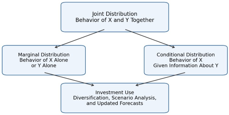
Figure 1 shows how the three views fit together. The joint distribution is the starting point because it describes how two variables behave together. From that joint view, an analyst can isolate one variable through a marginal distribution or update the distribution of one variable after observing the other through a conditional distribution. In portfolio work, this distinction is important: an asset can look attractive on a marginal basis but behave poorly under the specific conditions in which protection is needed most.

Marginal Density

For a continuous bivariate distribution, the marginal density of \(X_1\) is obtained by integrating the joint density over all possible values of \(X_2\):

$$
f_{X_1}(x_1) = \int_{-\infty}^{\infty} f_{X_1,X_2}(x_1, u_2) \, du_2
$$

Where:

• \(f_{X_1}(x_1)\) is the marginal density of \(X_1\) evaluated at \(x_1\)
• \(f_{X_1,X_2}(x_1, u_2)\) is the joint density of \(X_1\) and \(X_2\)
• \(u_2\) is the integration variable for \(X_2\)
• \(du_2\) indicates integration over very small changes in \(u_2\)
• The limits \(-\infty\) to \(\infty\) mean that all possible values of \(X_2\) are included

Similarly, the marginal density of \(X_2\) is:

Where:

• \(f_{X_2}(x_2)\) is the marginal density of \(X_2\) evaluated at \(x_2\)
• \(u_1\) is the integration variable for \(X_1\)
• All other terms follow the same meaning as defined above

The marginal distribution is useful when the analyst wants to understand one variable without conditioning on a particular value of the other. For example, the marginal distribution of a bond index return tells us how the bond index behaves overall. It does not tell us how the bond index behaves specifically when equities sell off, when inflation rises, or when policy rates are cut. For that, the analyst needs a conditional distribution.

$$ \textbf{Table 1: Joint, Marginal, and Conditional Views} \\
\begin{array}{l|c|c}
\textbf{View} & \textbf{Main Question Answered} & \textbf{Practical Finance Use} \\
\hline
\text{Joint distribution} & {\text{How do two variables behave} \\ \text{together?}} & {\text{Modeling co-movement between} \\ \text{asset returns}} \\
\hline
\text{Marginal distribution} & {\text{How does one variable behave} \\ \text{by itself?}} & {\text{Assessing one asset’s return} \\ \text{distribution in isolation}} \\
\hline
\text{Conditional distribution} & {\text{How does one variable behave given} \\ \text{information about another?}} & {\text{Scenario analysis, stress testing,} \\ \text{and forecast updating}} \\
\end{array}
$$

Table 1 is a useful way to organize the logic. Joint analysis starts with co-movement. Marginal analysis isolates one variable. Conditional analysis updates the forecast when additional information is known. In exam questions, many errors come from mixing up these three views.

Example 1: Joint and Marginal Probabilities in an Equity Screen

An equity analyst reviews 600 large‑cap companies. Of these, 150 are classified as artificial intelligence (AI) infrastructure firms and 450 as other firms. The analyst records whether each company outperformed the index over the past year as follows:

$$
\begin{array}{l|c|c|c}
\textbf{One-Year Relative Return} & \textbf{Other Firms} & \textbf{AI Infrastructure Firms} & \textbf{Total} \\
\hline
\text{Outperformed the index} & 135 & 75 & 210 \\
\hline
\text{Did not outperform the index} & 315 & 75 & 390 \\
\hline
\textbf{Total} & \bf{450} & bf{150} & bf{600} \\
\end{array}
$$

Using the above data, calculate:

1. The joint probability of selecting a firm that is both an AI infrastructure firm and an outperformer.
2. The marginal probability of selecting an AI infrastructure firm.
3. The marginal probability of selecting an outperformer.

Solution

Start by quoting the formula:

$$
P(A \cap B) = \frac{\text{Number of outcomes in both } A \text{ and } B}{\text{Total number of outcomes}}
$$

Where:

• \(P(A \cap B)\) is the joint probability that events \(A\) and \(B\) both occur
• \(A\) is one event of interest
• \(B\) is another event of interest
• \(A \cap B\) means the intersection of \(A\) and \(B\)

The joint probability of selecting a firm that is both an AI infrastructure firm and an outperformer is:

$$
P(\text{AI infrastructure} \cap \text{outperformed}) = \frac{75}{600} = 12.5\%
$$

The marginal probability of selecting an AI infrastructure firm is:

$$
P(\text{AI infrastructure}) = \frac{150}{600} = 25.0\%
$$

The marginal probability of selecting an outperformer is:

$$
P(\text{outperformed}) = \frac{210}{600} = 35.0\%
$$

The joint probability answers a different question from the marginal probabilities. The joint probability refers to both characteristics at once. The marginal probabilities describe each characteristic on its own.

Conditional Expectation

A conditional expectation is the expected value of a random variable given that a stated condition is true. It is a way of updating the expected value after information has been incorporated.

For a discrete random variable, the conditional expectation is:

$$
E[X|Y = y] = \sum_{x} x \times P(X = x|Y = y)
$$

Where:

• \(E[X|Y = y]\) is the expected value of \(X\) given that \(Y\) equals \(y\)
• \(X\) is the random variable being forecast
• \(Y\) is the conditioning random variable
• \(y\) is the observed or assumed value of \(Y\)
• \(x\) is a possible value of \(X\)
• \(P(X = x|Y = y)\) is the conditional probability that \(X\) equals \(x\) given \(Y = y\)
• \(\sum_{x}\) indicates summation over all possible values of \(X\)

For a continuous random variable, the conditional expectation is:

$$
E[X|Y = y] = \int_{-\infty}^{\infty} x f_{X|Y}(x|y) \, dx
$$

Where:

• \(f_{X|Y}(x|y)\) is the conditional density of \(X\) given \(Y = y\)
• \(dx\) indicates integration over very small changes in \(x\)
• All other terms have been defined above

The conditional expectation should be interpreted as a revised center of the distribution. It is not necessarily the most likely outcome. It is the probability-weighted average after the condition has been imposed.

Example 2: Conditional Expected Return After a Central Bank Decision

A strategist estimates the one‑month return on a bank equity index under three possible market reactions following a central bank rate decision. If the central bank cuts the policy rate by 25 basis points, the conditional probabilities and returns are given below.

$$
\begin{array}{l|c|c}
\textbf{Market Reaction if 25 bp Cut Occurs} & \textbf{Conditional Probability} & \textbf{Bank Equity Index Return} \\
\hline
\text{Relief rally} & 0.40 & 6.0\% \\
\hline
\text{Modest repricing} & 0.45 & 2.0\% \\
\hline
\text{Growth concern dominates} & 0.15 & -5.0\% \\
\end{array}
$$

Calculate the expected return of the bank equity index conditional on a 25 bp cut.

Solution

We know that:

$$
E[X|Y = y] = \sum_{x} x \times P(X = x|Y = y)
$$

Where:

• \(E[X|Y = y]\) is the expected bank equity return given a 25 bp policy rate cut
• \(X\) is the bank equity index return
• \(Y\) is the central bank decision
• \(y\) is a 25 bp policy rate cut
• \(x\) is a possible return outcome
• \(P(X = x|Y = y)\) is the probability of that return outcome conditional on the 25 bp cut

The conditional expected return is:

$$
\begin{align}
E[X|Y = 25\text{ bp cut}] &= (0.40 \times 6.0\%) + (0.45 \times 2.0\%) + (0.15 \times -5.0\%) \\
E[X|Y = 25\text{ bp cut}] &= 2.40\% + 0.90\% – 0.75\% = 2.55\%
\end{align}
$$

The 2.55% result is not the expected return for all possible central bank decisions. It is the expected return conditional on a 25 bp cut. If the central bank instead held rates steady or cut by 50 bps, the relevant conditional probabilities and return outcomes could be different.

Conditional Variance

A conditional mean tells the analyst the center of the distribution after a condition is imposed. The analyst also needs to know how uncertain the outcomes remain around that conditional center. That uncertainty is measured by conditional variance.

The conditional variance is:

$$
\text{Var}(X|Y = y) = E\left[\left(X – E[X|Y = y]\right)^2 \middle| Y = y\right]
$$

Where:

• \(\text{Var}(X|Y = y)\) is the variance of \(X\) conditional on \(Y = y\)
• \(E[X|Y = y]\) is the conditional expected value of \(X\)
• \(X – E[X|Y = y]\) is the deviation of \(X\) from its conditional mean
• The squared term measures dispersion around the conditional mean

An equivalent computational form is:

$$
\text{Var}(X|Y = y) = E\left[X^2 \middle| Y = y\right] – \left(E[X|Y = y]\right)^2
$$

Where:

• \(E\left[X^2 \middle| Y = y\right]\) is the conditional expected value of the squared outcome
• \(\left(E[X|Y = y]\right)^2\) is the square of the conditional mean

Conditional variance is especially important in stress testing. A condition may improve expected return but still leave a wide range of possible outcomes. Conversely, a condition may lower expected return but reduce uncertainty. Both the center and the dispersion matter.

Example 3: Conditional Variance of a Credit Index Return

A credit analyst models one‑month return on a short‑duration credit index conditional on a soft‑landing macro scenario. The conditional probabilities and returns are shown below.

$$
\begin{array}{l|c|c}
\textbf{Credit Market Outcome in a Soft Landing} & \textbf{Conditional Probability} & \textbf{Credit Index Return} \\
\hline
\text{Spreads tighten} & 0.30 & 4.0\% \\
\hline
\text{Carry dominates} & 0.50 & 2.0\% \\
\hline
\text{Mild spread widening} & 0.20 & -1.0\% \\
\end{array}
$$

Calculate the conditional mean, variance, and standard deviation of the credit index return.

Solution

We know that:

$$
\text{Var}(X|Y = y) = E\left[X^2 \middle| Y = y\right] – \left(E[X|Y = y]\right)^2
$$

Where:

• \(\text{Var}(X|Y = y)\) is the variance of the credit index return conditional on a soft landing
• \(X\) is the credit index return
• \(Y\) is the macro scenario
• \(y\) is the soft-landing scenario
• \(E\left[X^2 \middle| Y = y\right]\) is the conditional expected squared return
• \(E[X|Y = y]\) is the conditional expected return

First, calculate the conditional mean:

$$
E[X|Y = \text{soft landing}] = (0.30 \times 4.0\%) + (0.50 \times 2.0\%) + (0.20 \times -1.0\%) = 2.0\%
$$

Next, calculate the conditional expected squared return, using percentage returns:

$$
\begin{align}
E\left[X^2 \middle| Y = \text{soft landing}\right] &= (0.30 \times 4.0^2) + (0.50 \times 2.0^2) + (0.20 \times (-1.0)^2) \\
E\left[X^2 \middle| Y = \text{soft landing}\right] &= 4.80 + 2.00 + 0.20 = 7.00
\end{align}
$$

Finally, calculate conditional variance:

$$
\text{Var}(X|Y = \text{soft landing}) = 7.00 – 2.0^2 = 3.00
$$

The conditional variance is 3.00 percentage points squared. The conditional standard deviation is:

$$
\sqrt{3.00} = 1.73\%
$$

The expected return is positive, but there is still meaningful dispersion around that conditional mean.

The Total Probability Rule for Expected Value

Conditional expectations can be combined to recover an unconditional expected value when the conditions are mutually exclusive and exhaustive. Mutually exclusive means that only one condition can occur. Exhaustive means that the conditions cover all possible cases.

The total probability rule for expected value is:

$$
E[X] = \sum_{i=1}^{n} E[X|S_i]P(S_i)
$$

Where:

• \(E[X]\) is the unconditional expected value of \(X\)
• \(E[X|S_i]\) is the expected value of \(X\) conditional on scenario \(S_i\)
• \(P(S_i)\) is the probability of scenario \(S_i\)
• \(S_i\) is the ith scenario
• \(n\) is the number of mutually exclusive and exhaustive scenarios

This formula is the bridge between scenario analysis and a full forecast. Analysts often build expected returns by first estimating returns in separate states and then weighting those conditional forecasts by the probability of each state.

Example 4: From Conditional Returns to an Unconditional Expected Return

A multi‑asset team estimates conditional expected returns for a balanced portfolio under three economic scenarios. The probabilities and conditional returns are shown below.

$$
\begin{array}{l|c|c}
\textbf{Economic Scenario} & \textbf{Scenario Probability} & \textbf{Conditional Expected Portfolio Return} \\
\hline
\text{Hard landing} & 0.25 & -6.0\% \\
\hline
\text{Slow growth} & 0.45 & 4.0\% \\
\hline
\text{Productivity boom} & 0.30 & 12.0\% \\
\end{array}
$$

Calculate the unconditional expected portfolio return.

Solution

Start by quoting the formula:

$$
E[X] = \sum_{i=1}^{n} E[X|S_i]P(S_i)
$$

Where:

• \(E[X]\) is the unconditional expected portfolio return
• \(E[X|S_i]\) is the expected portfolio return conditional on scenario \(S_i\)
• \(P(S_i)\) is the probability of scenario \(S_i\)
• \(S_i\) represents each economic scenario
• \(n\) is the number of scenarios

The unconditional expected return is:

$$
\begin{align}
E[X] &= (-6.0\% \times 0.25) + (4.0\% \times 0.45) + (12.0\% \times 0.30) \\
E[X] &= -1.50\% + 1.80\% + 3.60\% = 3.90\%
\end{align}
$$

The unconditional expected return is 3.90%. This value is not tied to one particular scenario. It is the probability-weighted average of the conditional expected returns across all scenarios.

Conditional Covariance

Conditional covariance measures how two variables co-move under a specific condition. This is important because relationships between assets can change across regimes. Equity and bond returns may have one covariance in a disinflationary slowdown and a very different covariance during an inflation shock. That is why risk models based only on unconditional historical covariance can be misleading.

The conditional covariance is:

$$
\text{Cov}(X, Y|S) = E\left[\left(X – E[X|S]\right)\left(Y – E[Y|S]\right) \middle| S\right]
$$

Where:

• \(\text{Cov}(X, Y|S)\) is the covariance between \(X\) and \(Y\) conditional on scenario \(S\)
• \(X\) is the first random variable
• \(Y\) is the second random variable
• \(S\) is the conditioning scenario
• \(E[X|S]\) is the conditional expected value of \(X\)
• \(E[Y|S]\) is the conditional expected value of \(Y\)
• The product of deviations captures whether the two variables tend to move together under scenario \(S\)

An equivalent computational form is:

$$
\text{Cov}(X, Y|S) = E[XY|S] – E[X|S]E[Y|S]
$$

Where:

• \(E[XY|S]\) is the conditional expected value of the product of \(X\) and \(Y\)
• \(E[X|S]E[Y|S]\) is the product of the conditional expected values

The sign of conditional covariance is often more informative than its raw magnitude. A positive conditional covariance means the two variables tend to be above or below their conditional means together. A negative conditional covariance means one tends to be above its conditional mean when the other is below its conditional mean. The magnitude should be interpreted carefully because covariance depends on the units used.

Example 5: Conditional Covariance Under an Inflation Shock

A portfolio risk team analyzes equity and government bond returns conditional on an inflation‑shock scenario. Within that scenario, the team considers three possible market outcomes. The probabilities and returns are shown below.

$$
\begin{array}{l|c|c|c}
{\textbf{Inflation-Shock Outcome}} & {\textbf{Conditional} \\ \textbf{Probability}} & \textbf{Equity Return, X} & \textbf{Government Bond Return, Y} \\ \hline
\text{Severe repricing} & 0.30 & -12.0\% & -6.0\% \\ \hline
\text{Moderate repricing} & 0.50 & -5.0\% & -2.0\% \\ \hline
\text{Policy credibility restored} & 0.20 & 4.0\% & 1.0\% \\
\end{array}
$$

Calculate the conditional covariance between equity and bond returns.

Solution

Recall that:

$$
\text{Cov}(X, Y|S) = E[XY|S] – E[X|S]E[Y|S]
$$

Where:

• \(\text{Cov}(X, Y|S)\) is the covariance between equity and government bond returns conditional on an inflation shock
• \(X\) is the equity return
• \(Y\) is the government bond return
• \(S\) is the inflation-shock scenario
• \(E[XY|S]\) is the conditional expected product of equity and bond returns
• \(E[X|S]\) is the conditional expected equity return
• \(E[Y|S]\) is the conditional expected government bond return

First, calculate the conditional expected returns:

$$
\begin{align}
E[X|S] &= (0.30 \times -12.0\%) + (0.50 \times -5.0\%) + (0.20 \times 4.0\%) = -5.30\% \\
E[Y|S] &= (0.30 \times -6.0\%) + (0.50 \times -2.0\%) + (0.20 \times 1.0\%) = -2.60\%
\end{align}
$$

Next, calculate the conditional expected product, using percentage returns:

$$
E[XY|S] = (0.30 \times 72.0) + (0.50 \times 10.0) + (0.20 \times 4.0) = 27.40
$$

Finally, compute conditional covariance:

$$
\text{Cov}(X, Y|S) = 27.40 – (-5.30 \times -2.60) = 27.40 – 13.78 = 13.62
$$

The conditional covariance is 13.62 percentage points squared. The positive sign means that, within the inflation-shock scenario, equities and government bonds tend to move in the same direction relative to their conditional means. This is the kind of regime in which bonds may fail to provide the usual diversification benefit.

Conditional Forecasting Through a Probability Tree

A probability tree is a practical way to organize a forecast when an outcome unfolds over several stages. Each branch represents a possible event, each branch has an assigned probability, and each final node shows a possible terminal outcome. The value of the tree is not merely visual. It forces the analyst to make the sequence of assumptions explicit: what can happen first, what can happen next, and how each path changes the final forecast.

In finance, this framework is useful whenever prices, returns, defaults, cash flows, or policy decisions evolve through time. A credit analyst may use a tree to model rating migration and default. An equity analyst may use it to model a company’s share price after successive earnings announcements. A risk manager may use it to trace how a portfolio could behave after a sequence of interest rate changes. The common idea is that forecasts become more informative when they are stated conditionally: given what has already happened, what is the expected outcome from here?

The section below uses a three-period price tree.

Figure 2: Conditional Price Forecasting Through a Three-Period Probability Tree

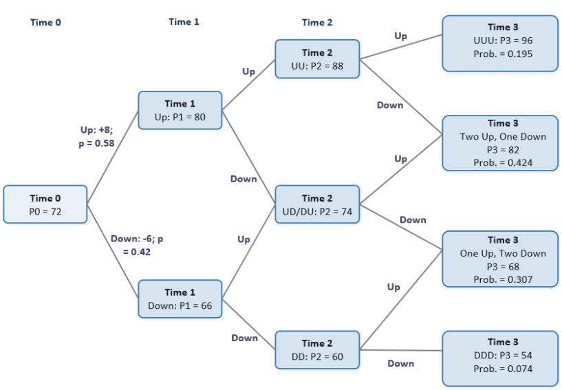
Figure 2 begins with an asset price of 72 at Time 0. In each period, the asset can move up by 8 with probability 0.58 or down by 6 with probability 0.42.

After three periods, there are four possible terminal prices: 96, 82, 68, and 54. The middle terminal prices can be reached through more than one path, so their probabilities are larger than the probability of any single path.

For example, a terminal price of 82 can occur after two upward moves and one downward move. There are three different orders in which that can happen: up-up-down, up-down-up, and down-up-up. The probability of one such path is the product of the branch probabilities. The total probability of the terminal price is the probability of one path multiplied by the number of paths that lead to that price.

The terminal probabilities are calculated as follows:

$$
P(P_3 = 96) = (0.58)^3 = 0.195
$$

$$
P(P_3 = 82) = 3(0.58)^2(0.42) = 0.424
$$

$$
P(P_3 = 68) = 3(0.58)(0.42)^2 = 0.307
$$

$$
P(P_3 = 54) = (0.42)^3 = 0.074
$$

Where:

• \(P_3\) is the asset price at Time 3
• \(P(P_3 = x)\) is the probability that the Time 3 price equals \(x\)
• 0.58 is the probability of an upward price move in any one period
• 0.42 is the probability of a downward price move in any one period
• The coefficient 3 appears when three different paths lead to the same terminal price

The four probabilities sum to 1, allowing the analyst to calculate an unconditional terminal price forecast.

$$
E[P_3] = \sum_{i} P(P_3 = p_i)p_i
$$

Where:

• \(E[P_3]\) is the unconditional expected asset price at Time 3
• \(p_i\) is the \(i\)th possible terminal price
• \(P(P_3 = p_i)\) is the probability of the \(i\)th terminal price
• The summation sign means summation across all terminal price outcomes

Applying the formula:

$$
E[P_3] = (0.195)(96) + (0.424)(82) + (0.307)(68) + (0.074)(54) = 78.36
$$

The unconditional forecast at Time 0 is therefore 78.36. That number is not a guaranteed price, and it need not equal one of the possible terminal prices. It is a probability-weighted forecast across all terminal outcomes.

Conditional Forecast after the First Price Move

The tree becomes especially useful after new information arrives. Suppose the first move is upward, so the asset price at Time 1 is 80. The analyst should no longer use the full tree from Time 0. The relevant forecast is now conditional on the first upward move having occurred.

Once the first upward move is known, only the upper branch of the tree remains relevant. From that point, there are two periods left. The conditional terminal outcomes are:

$$
\begin{array}{l|c|c}
\textbf{Remaining Two-Period Path} & \textbf{Terminal Price} & \textbf{Conditional Probability} \\
\hline
\text{Up, Up} & 96 & 0.3364 \\
\hline
\text{Up, Down or Down, Up} & 82 & 0.4872 \\
\hline
\text{Down, Down} & 68 & 0.1764 \\
\end{array}
$$

The probabilities are conditional because they apply only after the first upward move has already occurred. In other words, the analyst is standing at the Time 1 upper node and looking forward from there.

The conditional expected terminal price is calculated using:

$$
E[P_3|U_1] = \sum_{i} P(P_3 = p_i|U_1)p_i
$$

Where:

• \(E[P_3|U_1]\) is the expected Time 3 price given that the first move was upward
• \(U_1\) is the event that the first-period price move was upward
• \(P(P_3 = p_i|U_1)\) is the probability of terminal price \(p_i\) conditional on the first move being upward
• \(p_i\) is the \(i\)th possible terminal price after the first upward move
• The summation sign means summation across the remaining terminal outcomes

Applying the formula:

$$
E[P_3|U_1] = (0.3364)(96) + (0.4872)(82) + (0.1764)(68) = 84.24
$$

The conditional forecast of 84.24 is higher than the unconditional forecast of 78.36 because the first upward move has already occurred. The forecast has been updated to reflect the new state of the world.

Conditional Variance Around the Updated Forecast

A probability tree can also be used to estimate the dispersion of possible terminal prices around the conditional expected value. In this example, after the first upward move, the possible terminal prices are 96, 82, and 68. The conditional variance measures how widely those outcomes are spread around the conditional mean of 84.24.

Start by quoting the formula:

$$
\text{Var}(P_3|U_1) = E[P_3^2|U_1] – \left(E[P_3|U_1]\right)^2
$$

Where:

• \(\text{Var}(P_3|U_1)\) is the variance of the Time 3 price conditional on the first move being upward.
• \(E[P_3^2|U_1]\) is the conditional expected value of the squared terminal price.
• \(E[P_3|U_1]\) is the conditional expected terminal price.

First, calculate the conditional expected squared price:

$$
E[P_3^2|U_1] = (0.3364)(96^2) + (0.4872)(82^2) + (0.1764)(68^2) = 7,191.87
$$

Then calculate the variance:

$$
\text{Var}(P_3|U_1) = 7,191.87 – (84.24)^2 = 95.49
$$

The conditional standard deviation is:

$$
\sigma_{P_3|U_1} = \sqrt{95.49} = 9.77
$$

Where:

• \(\sigma_{P_3|U_1}\) is the standard deviation of the Time 3 price conditional on the first move being upward.
• \(\sqrt{95.49}\) is the square root of the conditional variance.

The interpretation is straightforward: after the first upward move, the updated expected terminal price is 84.24, and the conditional standard deviation is 9.77. The first piece tells the analyst the updated center of the distribution. The second indicates how much uncertainty remains around the updated forecast.

Why Probability Trees Matter in Investment Analysis

The main lesson is that a probability tree separates paths, probabilities, and outcomes. The same terminal price may be reached through several paths, and a conditional forecast must use only the paths that remain possible after new information has arrived.

This logic is particularly important in investment decisions because new information rarely arrives all at once. Earnings surprises, inflation releases, policy decisions, credit events, and liquidity shocks unfold over time. A probability tree provides the analyst with a disciplined structure for revising forecasts as events unfold.

A good exam answer should therefore do three things. First, identify the relevant node in the tree. Second, use the probabilities that apply from that node onward. Third, interpret the result as a conditional forecast, not as a certain outcome.

Table 2: Core Conditional Measures

$$
\begin{array}{l|c|c|c}
\textbf{Measure} & \textbf{Formula} & \textbf{Main Interpretation} & \textbf{Common Exam Trap} \\
\hline
\text{Conditional mean} & E[X|S] & {\text{Center of the distribution after} \\ \text{scenario } S \text{ is imposed}} & {\text{Using unconditional probabilities} \\ \text{instead of conditional probabilities}} \\
\hline
\text{Conditional variance} & \text{Var}(X|S) & {\text{Dispersion around the} \\ \text{conditional mean}} & {\text{Squaring deviations from the} \\ \text{unconditional mean}} \\
\hline
\text{Conditional covariance} & \text{Cov}(X,Y|S) & {\text{Co-movement of two variables} \\ \text{within scenario } S} & {\text{Assuming the unconditional relationship} \\ \text{still holds in every regime}} \\
\hline
\text{Total probability rule} & E[X] = \sum_{i} E[X|S_i]P(S_i) & {\text{Combines conditional expectations} \\ \text{into an unconditional expectation}} & {\text{Forgetting to weight by} \\ \text{scenario probabilities}} \\
\end{array}
$$

Table 2 brings the tools together. Conditional analysis is not a separate topic from mean, variance, and covariance. It is the same logic applied after information is known or assumed. The key is to use the correct probability distribution: once a condition is imposed, only the probabilities that apply under that condition should be used.

Interpretation and Evaluation

It is important to pay attention to all three verbs in the learning outcome: calculate, interpret, and evaluate. To calculate is to apply the conditional formulas correctly. To interpret is to explain what the result means economically. To evaluate is to judge whether the result is useful in the situation being analyzed.

A conditional expected return may be high but attached to a condition that is unlikely or poorly defined. A conditional variance may look low because the analyst has ignored important scenarios. A conditional covariance may suggest diversification benefits in ordinary markets but fail during the specific stress scenario that matters most. The examiner will often test whether candidates can recognize these limitations.

The best way to think about this learning outcome is simple: information changes the relevant distribution. Once the distribution changes, the mean, variance, and covariance can change as well.

Question

A portfolio analyst evaluates equity and bond returns conditional on a hawkish central bank surprise. Within that scenario, the analyst assigns the following probabilities to three market reactions.

$$
\begin{array}{c|c|c|c}
{\textbf{Market Reaction}\\ \textbf{Conditional on}\\ \textbf{a Hawkish Surprise}} & \textbf{Conditional Probability} & \textbf{Equity Return, } X & \textbf{Bond Return, } Y \\
\hline
\text{Severe selloff} & 0.20 & -8.0\% & -3.0\% \\
\hline
\text{Moderate repricing} & 0.50 & -3.0\% & -1.0\% \\
\hline
\text{Relief rally} & 0.30 & 2.0\% & 1.0\% \\
\end{array}
$$

The conditional covariance between equity and bond returns is closest to:

1. 4.90 percentage points squared
2. 6.90 percentage points squared
3. -4.90 percentage points squared

The correct answer is A.

Recall that:

$$
\text{Cov}(X, Y|S) = E[XY|S] – E[X|S]E[Y|S]
$$

Where:

• \(\text{Cov}(X, Y|S)\) is the covariance between equity and bond returns conditional on a hawkish central bank surprise
• \(X\) is the equity return
• \(Y\) is the bond return
• \(S\) is the hawkish central bank surprise scenario
• \(E[XY|S]\) is the conditional expected product of the equity and bond returns
• \(E[X|S]\) is the conditional expected equity return
• \(E[Y|S]\) is the conditional expected bond return

First, calculate the conditional expected equity return:

$$
E[X|S] = (0.20 \times -8.0\%) + (0.50 \times -3.0\%) + (0.30 \times 2.0\%) = -2.50\%
$$

Next, calculate the conditional expected bond return:

$$
E[Y|S] = (0.20 \times -3.0\%) + (0.50 \times -1.0\%) + (0.30 \times 1.0\%) = -0.80\%
$$

Then calculate the conditional expected product, using percentage returns:

$$
E[XY|S] = (0.20 \times 24.0) + (0.50 \times 3.0) + (0.30 \times 2.0) = 6.90
$$

Finally, compute conditional covariance:

$$
\text{Cov}(X,Y|S) = 6.90 – (-2.50 \times -0.80) = 6.90 – 2.00 = 4.90
$$

The conditional covariance is 4.90 percentage points squared. The positive sign indicates that, conditional on a hawkish central bank surprise, equities and bonds tend to move in the same direction relative to their conditional means.

B is incorrect because it stops at \(E[XY|S]\) and fails to subtract \(E[X|S]E[Y|S]\).

C is incorrect because it gives the correct magnitude with the wrong sign. The conditional covariance is positive, not negative.