Bootstrap Resampling in Finance: Estimating Uncertainty from Historical Data

Resampling

Resampling refers to the process of repeatedly drawing samples from the original observed sample to make statistical inferences about population parameters. There are two common methods: Bootstrap and jackknife. Here, we’ll focus on the Bootstrap method.

Bootstrap Resampling

Bootstrapping works by taking the original sample and drawing new samples from it over and over, each time putting every observation back before the next draw. The method effectively treats the sample as a stand-in for the entire population, whose true distribution is unknown.

Bootstrap resampling relies on computer simulations for statistical inference, bypassing the need for conventional analytical formulas such as z-statistics. The bootstrap technique is underpinned by a strategy that mirrors the random sampling process from a population to create a sampling distribution.

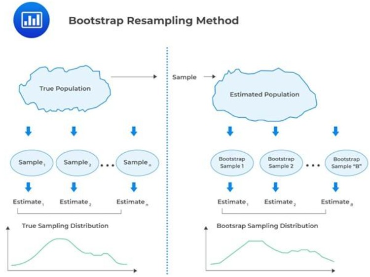
Note that in bootstrapping, we do not have information about the population. Our only insight comes from a sample of size drawn from this “unknown population.”

The key idea is simple: a randomly chosen sample can serve as a reasonable substitute for the whole population when the population itself cannot be observed directly. So, we can mimic drawing samples from the population by repeatedly resampling from the initial sample. Essentially, the bootstrap method treats the initially obtained sample as a stand-in for the entire population.

Bootstrapping vs. Historical Simulation

While both methods draw on observed data, they differ fundamentally. Historical simulation works directly with historical records, treating the past sequence of events as a fixed and complete representation of the population. Bootstrapping, by contrast, treats the observed sample as a stand-in for the population rather than assuming that the historical record fully captures it.

This distinction shapes how each method operates in practice:

• Bootstrapping repeatedly draws samples from the same dataset, with replacement, to build a simulated distribution of outcomes. It makes no assumptions about the shape of the underlying population.
• Historical simulation uses the historical dataset as-is, relying on the actual order and occurrence of past events without resampling.

Bootstrapping is especially useful when the true population distribution is not known, but the available sample is reasonably representative of what may occur in the future. In finance, the true distribution of asset returns is never known with certainty, which makes this flexibility particularly valuable. Compared to parametric methods, which typically assume normality and rely on historically derived standard deviations and correlations, bootstrapping imposes far fewer restrictions. This combination of flexibility and minimal assumptions makes it a robust tool for statistical inference and financial modelling.

Bootstrapping vs. Monte Carlo Simulation

Both bootstrap and Monte Carlo simulation techniques heavily rely on repetitive sampling. Bootstrap treats the resampled dataset as a proxy for the true population. It infers population parameters, such as the mean, variance, skewness, and kurtosis, from the statistical distribution of these samples.

Conversely, Monte Carlo simulation is centered on the generation of random data with a pre-determined statistical distribution of parameter values.

Simulation Using Bootstrapping

Simulation using bootstrapping is similar to Monte Carlo Simulation except for the source of random variables. In bootstrapping, the random variables are sampled from a bootstrap sample rather than from a probability distribution.
Consider the previous example:

Let’s say an investor wants to understand the potential outcomes of investing in a 70-30 stock-bond portfolio over 20 years.

The simulation steps using the bootstrap sampling distribution are as follows:

Step 1: Setup/parameterization

The quantity of interest here could be the final portfolio value after 20 years, denoted as \(V_{iT}\). The underlying variable is the portfolio’s return. The starting portfolio value is $100,000, with 70% invested in stocks and 30% in bonds.

Step 2: Scenario generation

Assume we’re interested in yearly returns, so the time horizon is 20 years. Divide the calendar time into sub-periods. In this case, we will assume yearly returns so that the number of subperiods is \(K = 20\), and time increment \(\Delta t\) is, therefore, one year.

Next, we use the historical return data as our empirical distribution. Instead of assuming that the annual portfolio return follows a specific theoretical distribution, we will use the bootstrap procedure to draw the \(K = 20\) yearly returns from the observed empirical distribution.

Step 3: Scenario evaluation/calculation engine

This step uses the bootstrap samples from Step 2 to compute the yearly changes in portfolio value. From there, we create a sequence of 20 portfolio values, starting with the initial value of $100,000.

The average portfolio value at the end of 20 years (\(V_{iT}\)) is calculated by summing up the portfolio values at the end of each year and dividing by 20. We then calculate the present value (\(V_{i0}\)) of this average value by discounting it to the present using an appropriate interest rate. The subscript \(i\) in \(V_{iT}\) and \(V_{i0}\) indicates that these values are from the ith bootstrap sample. This completes one bootstrap sample.

Step 4: Result compilation/analysis

We perform the simulation 1,000 times. We then calculate summary statistics, such as the mean, median, and percentiles of the distribution. \(V_{i0}\) of values. These summary statistics provide a range of potential outcomes for the portfolio value after 20 years, helping the investor understand the risks and rewards of the investment strategy based on the observed empirical return distribution.

Features of Bootstrapping Simulations

Bootstrapping serves as a useful complement to traditional analytical approaches in finance. Although it produces statistical estimates based on empirical distributions derived from historical price data, the results are approximations rather than exact values. When analytical solutions exist, they typically provide a better understanding of causal relationships and the fundamental drivers of a system.

The main benefit of bootstrapping is that it avoids imposing specific distributional assumptions. This becomes especially valuable when past patterns are likely to continue into the future, or when the true underlying distribution is too complex to be captured by standard parametric forms such as the normal or Student’s t distributions.

Advantages of Bootstrapping

A few prior assumptions: The method does not require any predetermined shape of the population distribution (e.g., normality). This flexibility makes it well-suited for situations where the real distribution is unknown or hard to specify.

Effective with small samples: Unlike many other techniques, bootstrapping performs reliably even with limited datasets. It can produce credible estimates of a statistic’s sampling variability from modest amounts of data.

Easy to understand and apply: The concept is simple—repeatedly draw observations from the existing sample, allowing each data point to be selected multiple times. This removes the need for complicated formulas or parametric models.

Reliable uncertainty measures: Bootstrapping yields solid estimates of standard errors and can build confidence intervals around statistics. This supports hypothesis testing and quantification of estimation risk. Compared to historical simulation, bootstrapping also diminishes the influence of extreme outliers.

Wide applicability: The technique works with nearly any statistic—mean, median, variance, correlation, and many others across diverse fields such as finance and biology, particularly when data structures are complex or non-parametric.

No requirement for a large external database: Unlike Monte Carlo or historical simulation, which either rely on theoretical distributions or extensive historical records, bootstrapping works directly from the sample at hand, making it ideal when data are scarce.

Disadvantages of Bootstrapping

Computationally heavy: Although conceptually simple, bootstrapping can require substantial processing power, especially when running many thousands of resamples. This may lead to long computation times, particularly with large datasets or when evaluating multiple statistics simultaneously.

Dependent on sample quality: Bootstrapping assumes that the available sample accurately represents the broader population. If the sample is biased or unrepresentative, the bootstrap outcomes will be misleading because the method magnifies any existing flaws.

Poor handling of time-series autocorrelation: Bootstrapping breaks the natural temporal dependencies (autocorrelation) often present in financial time series. For such data, specialized resampling techniques that preserve the order of observations may be necessary.

Cannot go beyond the observed range: Bootstrapping cannot generate scenarios that fall outside the minimum or maximum values present in the original dataset. When analyzing tail risks or hypothetical extreme events, methods like Monte Carlo simulation are more appropriate.

No theoretical explanation: Bootstrapping is entirely empirical. It does not provide insight into why the data behave as they do or offer a theoretical understanding of the underlying process. It is useful for estimation but not for explaining causality.

Question

Which of the following statements is most likely accurate in relation to bootstrap analysis?

1. Bootstrap analysis aims to deduce statistics about population parameters from a singular sample.
2. Bootstrap analysis involves the repeated extraction of samples of equal size, with replacement, from the initial population.
3. During bootstrap analysis, analysts must determine probability distributions for the primary risk factors governing the underlying random variables.

Solution

The correct answer is A.

The bootstrap analysis employs random sampling to generate an observed variable from a set of unknown population parameters. Although the actual distribution of the population is unknown to the analyst, the parameters of the population can be inferred through the sample produced via random sampling.

B is incorrect. In bootstrap analysis, the analyst repeatedly samples from the initial sample rather than the entire population. Each resample has the same size as the original sample, and for each new draw, selected items go back into the sample.

C is incorrect. During bootstrap analysis, analysts utilize the empirical distribution of the observed underlying variables. In contrast, the analyst must establish probability distributions for the key risk factors that govern the underlying variables in a Monte Carlo simulation.