Unconditional Expected Values in Finance: Mean, Variance, and Covariance

Introduction to Random Variables

A random variable assigns a numerical value to an uncertain outcome. In finance, the random variable might be a stock return next month, the number of defaults in a bond portfolio, the return on a cryptocurrency strategy, or the change in an economic indicator after a central bank announcement.

A random variable may be discrete or continuous. A discrete random variable has outcomes that can be counted. Examples include a credit rating score, the number of defaults in a portfolio, or the number of successful trades generated by an algorithm during a day. A continuous random variable can take infinitely many values within a range. Examples include a daily equity return, a change in bond yield, or a foreign exchange return.

The distinction matters because discrete and continuous variables are described differently. A discrete variable assigns probability to exact outcomes. A continuous variable assigns probability to intervals, because the probability of observing one exact value is effectively zero.

Figure 1: Discrete Probability Mass Function and Stepwise Cumulative Distribution Function

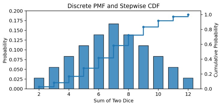
Figure 1 uses the sum of two dice to show the natural shape of a discrete distribution. The bars represent the probability mass function, which assigns probability to each exact outcome. The line represents the cumulative distribution function, which adds probabilities from left to right. Notice that the cumulative distribution rises in steps rather than as a smooth curve. That stepwise pattern is the signature of a discrete random variable: probability appears only at the possible outcomes, and the cumulative probability jumps only when one of those outcomes is reached.

The same logic applies when an analyst models the number of defaults in a pool of loans, the number of stocks that breach a risk limit, or the number of days in a month when a trading strategy generates a positive return. The outcomes are countable, so the probability model must assign probability to exact values.

Figure 2: Continuous Probability Density Function and Smooth Cumulative Distribution Function

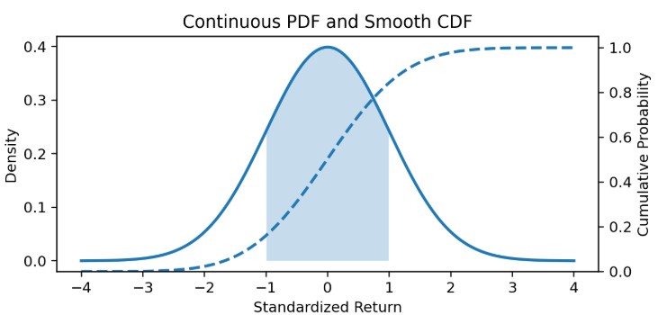
Figure 2 shows the corresponding picture for a continuous variable, such as a daily standardized return. The solid curve is a probability density function. It does not give the probability of one exact return. Instead, probability is represented by the area under the curve over a range of values. The dashed curve is the cumulative distribution function. Unlike the discrete CDF in Figure 1, the CDF in Figure 2 rises smoothly because the random variable can take many possible values along the number line.

This distinction is crucial in investment work. If a risk manager asks for the probability that a portfolio’s return falls between -1% and +1%, the answer comes from the area under the density curve over that interval. The shaded region in Figure 2 illustrates this idea. It is the interval, not a single point, that carries probability for a continuous variable.

Distribution Functions

A random variable is described by a function that maps outcomes to probabilities. The most general of these is the cumulative distribution function.

The cumulative distribution function is:

$$F(x) = P(X \le x)$$

Where:

• \(F(x)\) is the cumulative distribution function evaluated at \(x\)
• \(P(\cdot)\) is the probability of the event in parentheses
• \(X\) is the random variable
• \(x\) is a specific value on the number line
• \(X \le x\) is the event that the random variable takes a value less than or equal to \(x\)

The CDF answers questions such as:

• What is the probability that a monthly return is no more than (at most) 2%?
• What is the probability that losses do not exceed a particular threshold?
• What is the probability that a credit score falls below a certain level?

For a continuous random variable, probability over an interval is calculated using the probability density function:

$$P(a \le X \le b) = \int_{a}^{b} f_x(x) \, dx = F(b) – F(a)$$

Where:

• \(a\) is the lower bound of the interval
• \(b\) is the upper bound of the interval
• \(f_x(x)\) is the probability density function of \(X\) evaluated at \(x\)
• \(dx\) indicates integration over very small changes in \(x\)
• \(F(a)\) and \(F(b)\) are the cumulative probabilities at \(a\) and \(b\), respectively

The total probability under a continuous density must equal 1:

$$\int_{-\infty}^{\infty} f_x(x) \, dx = 1$$

Where:

• \(-\infty\) and \(\infty\) indicate that the integral is taken over the full range of possible values.
• 1 represents total probability across all possible outcomes.

For a discrete random variable, probability is added rather than integrated:

$$P(a \le X \le b) = \sum_{x=a}^{b} P(X = x)$$

Where:

• \(\sum\) indicates summation across all possible discrete values from \(a\) to \(b\).
• \(P(X = x)\) is the probability that the random variable is exactly equal to \(x\).

The probabilities across all possible discrete outcomes must also add to 1:

$$\sum_{x} P(X = x) = 1$$

Where:

• \(\sum_{x}\) means that probabilities are summed over every possible value of \(X\).

$$ \textbf{Table 1: Distribution Functions by Type of Random Variable} \\
\begin{array}{l|l|l|l}
\textbf{Type of} & \textbf{Function Used} & \textbf{What the Function} & \textbf{Example} \\
\textbf{Random} & & \textbf{Tells the Analyst} & \\
\textbf{Variable} & & & \\
\hline
\text{Discrete} & \text{Probability mass} & \text{Probability of each exact} & \text{Number of defaults in a credit} \\
& \text{function} & \text{outcome} & \text{portfolio} \\
\hline
\text{Discrete} & \text{Cumulative} & \text{Probability that the outcome} & \text{Probability that no more than} \\
& \text{distribution} & \text{is less than or equal to a} & \text{five loans default} \\
& \text{function} & \text{value} & \\
\hline
\text{Continuous} & \text{Probability density} & \text{How probability is} & \text{Distribution of daily equity} \\
& \text{function} & \text{distributed across intervals} & \text{returns} \\
\hline
\text{Continuous} & \text{Cumulative} & \text{Probability that the outcome} & \text{Probability that a portfolio loss} \\
& \text{distribution} & \text{is less than or equal to a} & \text{is no more than a specified} \\
& \text{function} & \text{value} & \text{amount} \\
\end{array}
$$

Table 1 ties the functions to practical use. The important point is that a PMF or PDF is not just a mathematical object. It tells the analyst how probability is spread across possible outcomes. Once that probability structure is understood, expected value, variance, and covariance can be calculated.

Unconditional Mean

The unconditional mean, also called the expected value, is the probability-weighted average of all possible outcomes. It is unconditional because no special condition or scenario has been imposed first. The analyst considers the full set of possible outcomes and weights each by its probability.

For a discrete random variable, the unconditional mean is:

$$\mu_X = E[X] = \sum_{i} x_i P(x_i)$$

Where:

• \(\mu_X\) is the unconditional mean of random variable \(X\)
• \(E[X]\) is the expected value of \(X\)
• \(x_i\) is the value of the \(i\text{th}\) possible outcome.
• \(P(x_i)\) is the probability of the \(i\text{th}\) possible outcome
• \(\sum_{i}\) indicates summation over all possible outcomes

For a continuous random variable, the unconditional mean is:

$$\mu_X = E[X] = \int_{-\infty}^{\infty} x f_X(x) \, dx$$

Where:

• \(x\) is a possible value of the continuous random variable
• \(f_X(x)\) is the probability density function of \(X\)

The mean should not be interpreted as the most likely outcome unless the distribution has that property. In many investment settings, the expected value may serve as a useful center of gravity even if no actual outcome matches it. A stock analyst may forecast a 6.8% expected return even though the realized return will almost certainly be something else.

Example 1: Expected Return Across Economic Regimes

Suppose that a strategist assigns probabilities to four economic regimes for the next year as follows:

$$
\begin{array}{l|c|c}
\textbf{Economic Regime} & \textbf{Probability} & \textbf{Equity Index Return} \\ \hline
\text{Recession} & 0.20 & -12.0\% \\ \hline
\text{Slow growth} & 0.30 & 2.0\% \\ \hline
\text{Stable expansion} & 0.35 & 9.0\% \\ \hline
\text{Strong growth} & 0.15 & 18.0\% \\
\end{array}
$$

Calculate the return on a broad equity index in each regime.

Solution

We know that:

$$\mu_X = E[X] = \sum_{i} x_i P(x_i)$$

The expected return is:

$$ \begin{align*}
E[X]&=-12.0\% (0.20)+2.0\%(0.30)+9.0\%(0.35)+18.0\%(0.15) \\
E[X] & =-2.40\%+0.60\%+3.15\%+2.70\%=4.05\%
\end{align*} $$

The unconditional expected return is 4.05%. This is not a promise that the index will earn 4.05%. It is the probability-weighted average return across all the regimes in the strategist’s forecast.

Unconditional Variance and Standard Deviation

The mean tells us the center of the distribution, but investment risk also depends on how widely outcomes are dispersed around that center. The unconditional variance measures the average squared deviation from the mean.

The unconditional variance is:

$$\sigma_X^2 = Var(X) = E\left[(X – E[X])^2\right] = E[X^2] – (E[X])^2$$

Where:

• \(\sigma_X^2\) is the variance of \(X\)
• \(Var(X)\) is another notation for the variance of \(X\)
• \(E\left[(X – E[X])^2\right]\) is the expected squared deviation from the mean
• \(E[X^2]\) is the expected value of the squared outcome
• \((E[X])^2\) is the square of the expected value

The standard deviation is the square root of the variance:

$$\sigma_X = \sqrt{Var(X)}$$

Where:

• \(\sigma_X\) is the standard deviation of \(X\)
• \(\sqrt{\cdot}\) denotes the square root

Variance is useful mathematically, but standard deviation is often easier to interpret because it is expressed in the same units as the variable itself. If the random variable is a percentage return, the standard deviation is also expressed in percentage points.

Example 2: Variance and Standard Deviation of Returns

Using the same regime forecast from Example 1, calculate the variance and standard deviation of the equity index return.

Solution

We know that:

$$\sigma_X^2 = Var(X) = E[X^2] – (E[X])^2$$

The expected return from Example 1 is \(E[X] = 4.05\%\). First calculate \(E[X^2]\):

\begin{align*}
E[X^2] &= (0.20)(-12.0)^2 + (0.30)(2.0)^2 + (0.35)(9.0)^2 + (0.15)(18.0)^2 \\
E[X^2] &= 28.80 + 1.20 + 28.35 + 48.60 = 106.95
\end{align*}

Then subtract the square of the expected return:

$$Var(X) = 106.95 – (4.05)^2 = 106.95 – 16.4025 = 90.5475$$

The standard deviation is:

$$\sigma_X = \sqrt{90.5475} = 9.52\%$$

The variance is 90.5475 percentage points squared, and the standard deviation is 9.52%. The standard deviation provides a more intuitive risk measure: returns are expected to vary meaningfully around the 4.05% expected return.

Unconditional Covariance

The unconditional covariance measures whether two random variables tend to move together. A positive covariance means that high values of one variable tend to occur with high values of the other, and low values tend to occur together. A negative covariance means that one variable tends to be above its mean when the other is below its mean.

The unconditional covariance is:

$$\sigma_{XY} = Cov(X,Y) = E\left[(X – E[X])(Y – E[Y])\right] = E[XY] – E[X]E[Y]$$

Where:

• \(\sigma_{XY}\) is the covariance between \(X\) and \(Y\)
• \(Y\) is a second random variable.
• \(E[Y]\) is the expected value of \(Y\)
• \(E[XY]\) is the expected value of the product of \(X\) and \(Y\)
• \(E[X]E[Y]\) is the product of the two expected values

Covariance is central to portfolio construction because it captures co-movement. Two risky assets can still reduce portfolio risk if their returns do not move together strongly. A defensive bond allocation, for example, may be valuable not only because of its own expected return but also because of how it behaves when equity returns are weak.

Covariance, however, is not standardized. Its numerical size depends on the units used. A covariance expressed using percentage returns will look different from one expressed using decimal returns. For assessing the strength of a relationship, correlation is often more intuitive, but covariance is the building block used to compute portfolio variance.

Example 3: Covariance Between Equity and Bond Returns

An analyst estimates returns for an equity index and a government bond index under four macroeconomic regimes as follows:

$$
\begin{array}{l|c|c|c}
\textbf{Economic Regime} & \textbf{Probability} & \textbf{Equity Return, } X & \textbf{Bond Return, } Y \\ \hline
\text{Recession} & 0.25 & -10.0\% & 6.0\% \\ \hline
\text{Slow growth} & 0.30 & 1.0\% & 4.0\% \\ \hline
\text{Stable expansion} & 0.30 & 8.0\% & 2.0\% \\ \hline
\text{Inflation scare} & 0.15 & 12.0\% & -3.0\% \\
\end{array}
$$

Calculate the covariance between X and Y.

Solution

We know that:

$$\sigma_{XY} = Cov(X,Y) = E[XY] – E[X]E[Y]$$

First, calculate the expected return for each index:

$$
\begin{align*}
E[X] &= (0.25)(-10.0) + (0.30)(1.0) + (0.30)(8.0) + (0.15)(12.0) = 2.00\% \\
E[Y] &= (0.25)(6.0) + (0.30)(4.0) + (0.30)(2.0) + (0.15)(-3.0) = 2.85\%
\end{align*}
$$

Next calculate \(E[XY]\):

$$
\begin{align*}
E[XY] &= (0.25)(-10.0)(6.0) + (0.30)(1.0)(4.0) + (0.30)(8.0)(2.0) + (0.15)(12.0)(-3.0) \\
E[XY] &= -15.00 + 1.20 + 4.80 – 5.40 = -14.40
\end{align*}
$$

Now compute covariance:

$$Cov(X, Y) = -14.40 – (2.00)(2.85) = -20.10$$

The covariance is -20.10 percentage points squared. The negative sign is the key interpretation: in this scenario design, stronger equity outcomes tend to be associated with weaker bond outcomes, and weak equity outcomes tend to be associated with stronger bond outcomes. That pattern is exactly why bonds may help cushion a diversified portfolio in some equity selloffs.

$$ \textbf{Table 2: Core Unconditional Measures} \\
\begin{array}{l|c|l|l}
\textbf{Measure} & \textbf{Formula} & \textbf{Main Interpretation} & \textbf{Common Exam Trap} \\ \hline
\text{Mean} & E[X] = \sum_{i} x_i P(x_i) & \begin{array}{l} \text{Probability-weighted center} \\ \text{of the distribution} \end{array} & \begin{array}{l} \text{Treating the mean as the most} \\ \text{likely outcome} \end{array} \\ \hline
\text{Variance} & Var(X) = E[X^2] – (E[X])^2 & \begin{array}{l} \text{Squared dispersion around} \\ \text{the mean} \end{array} & \begin{array}{l} \text{Forgetting to subtract the square} \\ \text{of the mean} \end{array} \\ \hline
\begin{array}{l} \text{Standard} \\ \text{deviation} \end{array} & \sigma_X = \sqrt{Var(X)} & \begin{array}{l} \text{Dispersion in the original} \\ \text{units} \end{array} & \begin{array}{l} \text{Confusing variance with} \\ \text{standard deviation} \end{array} \\ \hline
\text{Covariance} & Cov(X,Y) = E[XY] – E[X]E[Y] & \begin{array}{l} \text{Direction of co-movement} \\ \text{between two variables} \end{array} & \begin{array}{l} \text{Interpreting a large covariance} \\ \text{as strong without considering} \\ \text{units} \end{array} \\
\end{array}
$$

Table 2 summarizes the core tools in this LO. In exam questions, the calculations are usually straightforward once the structure is recognized. The harder part is often interpretation. As a candidate, you should always ask yourself one simple question: Am I calculating a center, a spread, or a co-movement?

The Law of Large Numbers

The law of large numbers states that as the number of independent observations increases, the sample mean tends to converge to the true population mean, provided the sample is representative. This is why analysts usually trust a well-constructed sample of many observations more than a tiny sample.

In finance, this principle must be used carefully. A larger sample is helpful only if the data are relevant and representative. A long history of returns may be less useful if the market structure has changed, if monetary policy regimes have shifted, or if the asset class is new and dominated by a short period of unusual conditions. The law of large numbers supports statistical inference, but it does not rescue a poorly chosen sample.

Figure 3: Sample Mean Converging Toward the Unconditional Mean

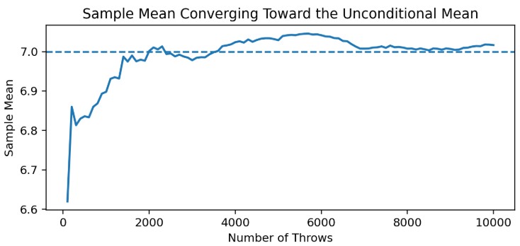
Figure 3 illustrates the law of large numbers using repeated throws of two dice. Early in the simulation, the sample mean moves around because each additional observation has a large effect on the average. As the number of observations increases, the sample mean becomes more stable and approaches the unconditional mean of 7. The financial parallel is direct: a small sample of recent returns may be noisy, whereas a larger, more representative sample can yield a more stable estimate of the expected value.

The figure should not be read as saying that more data always means better analysis. If the data come from a period that no longer reflects the current investment environment, adding more observations may create a false sense of comfort. As an analyst, you still need judgment about whether the sample reflects the population being modeled.

Example 4: Interpreting the Law of Large Numbers in a Market Context

A quant researcher back-tests a short-term equity signal using 25 trades and finds an average return of 0.80% per trade. After expanding the test to 2,500 trades across several market environments, the average return falls to 0.18% per trade.

The law of large numbers helps explain why the smaller estimate may have been unreliable. With only 25 trades, a few unusually profitable outcomes can dominate the average. With 2,500 trades, the sample mean is less sensitive to any one outcome and may be closer to the signal’s true expected return, provided that the broader sample is representative.

This is a common real-world problem. A strategy that appears impressive in a narrow back-test may become ordinary once tested across different volatility regimes, sectors, and liquidity conditions.

Interpretation and Evaluation

It’s very important to pay attention to the wording of the learning outcome statement in this case. To calculate means applying the formulas correctly. To interpret means explaining the economic meaning of the result. To evaluate means judging whether the measure is useful in context.

For example, a high expected return is not automatically attractive if the variance is also very high. A negative covariance is not automatically good unless it helps the portfolio in the states where protection is needed. A historical average is not automatically a reliable expected value if past samples do not represent the future investment environment.

Good analysts combine computation with judgment. In practice, the numbers are only the beginning of the analysis.

Question

A portfolio analyst models next year’s returns for an equity index and a short-duration credit index under four possible market regimes.

$$
\begin{array}{l|c|c|c}
\textbf{Market Regime} & \textbf{Probability} & \textbf{Equity Index Return, } X & \textbf{Credit Index Return, } Y \\ \hline
\text{Hard landing} & 0.25 & -8.0\% & 3.0\% \\ \hline
\text{Slow growth} & 0.35 & 2.0\% & 2.0\% \\ \hline
\text{Soft landing} & 0.25 & 9.0\% & 1.0\% \\ \hline
\text{Productivity boom} & 0.15 & 18.0\% & -1.0\% \\
\end{array}$$

The unconditional covariance between the equity index return and the credit index return is closest to:

1. -10.71 percentage points squared
2. -5.05 percentage points squared
3. 10.71 percentage points squared

The correct answer is A.

$$\sigma_{XY} = Cov(X, Y) = E[XY] – E[X]E[Y]$$

Where:

• \(\sigma_{XY}\) is the covariance between random variables \(X\) and \(Y\)
• \(Cov(X, Y)\) is another notation for covariance
• \(X\) is the equity index return
• \(Y\) is the credit index return
• \(E[XY]\) is the expected value of the product of the equity and credit returns
• \(E[X]\) is the expected equity index return
• \(E[Y]\) is the expected credit index return

First calculate \(E[X]\):

$$E[X] = (0.25)(-8.0) + (0.35)(2.0) + (0.25)(9.0) + (0.15)(18.0) = 3.65\%$$

Then calculate \(E[Y]\):

$$E[Y] = (0.25)(3.0) + (0.35)(2.0) + (0.25)(1.0) + (0.15)(-1.0) = 1.55\%$$

Next calculate \(E[XY]\):

$$
\begin{align*}
E[XY] &= (0.25)(-8.0)(3.0) + (0.35)(2.0)(2.0) + (0.25)(9.0)(1.0) + (0.15)(18.0)(-1.0) \\
E[XY] &= -6.00 + 1.40 + 2.25 – 2.70 = -5.05
\end{align*}
$$

Finally, calculate covariance:

$$Cov(X, Y) = -5.05 – (3.65)(1.55) = -10.7075$$

The covariance is approximately -10.71 percentage points squared, or -0.001071. The negative sign indicates that, in this scenario, stronger equity outcomes are associated with lower credit index returns, whereas weaker equity outcomes are associated with higher credit index returns.

B is incorrect because it stops at \(E[XY]\) and fails to subtract \(E[X]E[Y]\).

C is incorrect because it uses the correct magnitude but the wrong sign. The covariance is negative, not positive.