Optimal Portfolio Selection: Risk Aversion, Capital Allocation Line, Market Portfolio, and Capital Market Line

Why Optimal Portfolio Selection Starts With the Investor

Portfolio theory is sometimes presented as if there is one best portfolio for everyone. That is not the right intuition. The optimal portfolio depends on both the investment opportunity set and the investor’s willingness to bear risk. Two investors may agree on expected returns, variances, and correlations, yet choose different portfolios because one investor is more risk averse than the other.

The first two learning outcomes in this module showed how portfolio return and risk are calculated and how the efficient frontier identifies portfolios that are not dominated. This learning outcome asks the next question: once efficient portfolios are available, how does an investor choose among them?

The answer comes from combining three ideas. First, investors have risk preferences that can be summarized using a utility framework. Second, the presence of a risk-free asset creates a straight-line investment opportunity called the capital allocation line. Third, when the risky portfolio used in that line is the market portfolio, the capital allocation line becomes the capital market line, which provides the foundation for the capital asset pricing model.

Key Assumptions Behind the Framework

The theory works from simplifying assumptions. These assumptions are not intended to describe every real-world detail. They allow the model to isolate the relationship between risk, return, and investor preferences.

$$ \textbf{Table 1: Key Assumptions in Optimal Portfolio Selection} \\
\begin{array}{l|l|l}
\textbf{Assumption} & \textbf{Meaning} & \textbf{Why It Matters} \\
\hline
\text{Investors are rational and risk} & \text{Investors prefer higher expected} & \text{Portfolio choice can be modeled as} \\
\text{averse} & \text{return and lower risk, all else equal} & \text{utility maximization} \\ \hline
\text{Investors use a single-period} & \text{The portfolio is chosen now and} & \text{Risk and return can be compared} \\
\text{horizon} & \text{evaluated at the end of one period} & \text{over one common horizon} \\ \hline
\text{Investors can borrow and lend at} & \text{The risk-free asset has no return} & \text{A straight-line opportunity set can} \\
\text{the risk-free rate} & \text{volatility and is available to} & \text{be formed with a risky portfolio} \\
& \text{investors} & \\ \hline
\text{Taxes and transaction costs are} & \text{Trading and rebalancing are} & \text{The model focuses on pure} \\
\text{ignored} & \text{assumed frictionless} & \text{risk-return trade-offs} \\ \hline
\text{Investors share expectations} & \text{Investors agree on expected} & \text{The same efficient risky portfolio} \\
& \text{returns, variances, and} & \text{can be analyzed across investors} \\
& \text{covariances} & \\
\end{array}
$$

Table 1 should be interpreted as a model setup, not a promise about real markets. In practice, investors face taxes, transaction costs, borrowing constraints, short-sale constraints, behavioral biases, and imperfect information. These complications matter, but they do not eliminate the value of the framework. They explain why the framework should be applied with judgment.

Risk Preferences and Risk Aversion

Risk preference describes an investor’s attitude toward uncertainty. Investors are usually grouped into three broad categories.

A risk-seeking investor prefers an uncertain payoff to a certain payoff with the same expected value. A risk-neutral investor is indifferent between the two. A risk-averse investor prefers the certain payoff when the expected values are equal.

Most investment models assume that investors are risk averse. That assumption is realistic for long-term portfolio construction: investors generally require compensation for accepting volatility, drawdowns, and the possibility of failing to meet goals.

Figure 1: Investor Risk Preferences}

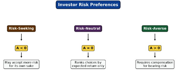
Figure 1 summarizes the three risk-preference cases. The coefficient of risk aversion, A, is positive for risk-averse investors, zero for risk-neutral investors, and negative for risk-seeking investors. For CFA Level I portfolio selection, the most important case is risk aversion: the investor wants higher expected return but dislikes additional risk.

Utility and Portfolio Ranking

A simple utility function used in mean-variance analysis is:

$$U = E(r) – \frac{1}{2} A \sigma^2$$

Where:

• \(U\) is the investor’s utility score
• \(E(r)\) is the expected return of the portfolio
• \(A\) is the investor’s coefficient of risk aversion
• \(\sigma^2\) is the variance of portfolio returns

The equation says that utility rises with expected return and falls with risk. The penalty for risk is larger when the investor’s coefficient of risk aversion is higher. A more risk-averse investor therefore needs more additional expected return to accept the same increase in variance.

The mean-variance utility relationship can also be written generally as:

$$U_P = U(E(r_P), \sigma_P)$$

Where:

• \(U_P\) is the utility of portfolio \(P\)
• \(E(r_P)\) is the expected return of portfolio \(P\)
• \(\sigma_P\) is the standard deviation of portfolio \(P\)

This expression emphasizes that portfolio choice is a function of both return and risk. A portfolio with a higher expected return is not automatically better if the additional return is not sufficient compensation for the additional risk.

Example 1: Ranking Portfolios Using Utility

Assume we have three candidate portfolios for a risk-averse investor. The investor’s coefficient of risk aversion is 4, and the candidate portfolios have the following expected returns and standard deviations:

$$ \begin{array}{l|c|c}
\textbf{Portfolio} & \textbf{Expected Return} & \textbf{Standard Deviation} \\
\hline
\text{Defensive Income} & 7.0\% & 8.0\% \\ \hline
\text{Global Balanced} & 10.0\% & 15.0\% \\ \hline
\text{Growth Equity} & 13.0\% & 22.0\% \\
\end{array}
$$

Identify the portfolio with the highest utility for this investor.

Solution

Start by quoting the utility formula:

$$U = E(r) – \frac{1}{2} A \sigma^2$$

Where:

• \(U\) is the investor’s utility score
• \(E(r)\) is the expected return of the portfolio
• \(A = 4\) is the investor’s coefficient of risk aversion
• \(\sigma\) is the portfolio standard deviation
• \(\sigma^2\) is the portfolio variance

Using returns and standard deviations in decimal form:

$$\begin{align*}
U_{\text{Defensive Income}} &= 0.070 – \frac{1}{2}(4)(0.080)^2 = 0.0572 \\
U_{\text{Global Balanced}} &= 0.100 – \frac{1}{2}(4)(0.150)^2 = 0.0550 \\
U_{\text{Growth Equity}} &= 0.130 – \frac{1}{2}(4)(0.220)^2 = 0.0332
\end{align*}$$

The Defensive Income portfolio has the highest utility. Although it has the lowest expected return, its lower risk is valuable to a highly risk-averse investor. This is the central point of utility analysis: the optimal choice is not necessarily the portfolio with the highest expected return.

Indifference Curves

An indifference curve shows combinations of expected return and risk that provide the same utility to a particular investor. Every point on the same indifference curve is equally attractive to that investor.

For a risk-averse investor, indifference curves slope upward in risk-return space. More risk must be compensated by more expected return. A more risk-averse investor has steeper indifference curves because that investor requires more additional expected return for each additional unit of risk.

In portfolio selection, the investor wants the highest attainable indifference curve. The optimal portfolio is the point at which the best attainable investment opportunity just touches, or is tangent to, the investor’s indifference curve.

The Risk-Free Asset and Risky Portfolio Combinations

A risk-free asset has no return volatility over the relevant horizon. In practice, short-term government securities are often used as approximations, although they are not perfectly risk free in every currency, time horizon, or inflation-adjusted setting.

When an investor combines a risk-free asset with a risky portfolio, the expected return is:

$$E(r_c) = w_f r_f + (1 – w_f) E(r_Q)$$

Where:

• \(E(r_c)\) is the expected return of the combined portfolio
• \(w_f\) is the weight invested in the risk-free asset
• \(r_f\) is the risk-free rate
• \(1 – w_f\) is the weight invested in the risky portfolio
• \(E(r_Q)\) is the expected return of the risky portfolio \(Q\)

Because the risk-free asset has zero standard deviation and zero covariance with the risky portfolio, the combined portfolio’s standard deviation is:

$$\sigma_c = (1 – w_f) \sigma_Q$$

Where:

• \(\sigma_c\) is the standard deviation of the combined portfolio
• \(1 – w_f\) is the weight invested in the risky portfolio
• \(\sigma_Q\) is the standard deviation of the risky portfolio \(Q\)

This relationship is linear. The more the investor allocates to the risky portfolio, the higher both expected return and standard deviation become. If the investor borrows at the risk-free rate to invest more than 100% in the risky portfolio, expected return and risk both rise beyond the risky portfolio’s own return and risk.

The Capital Allocation Line

The capital allocation line, or CAL, shows all portfolios that can be formed by combining a risk-free asset with a chosen risky portfolio. Its equation is:

$$E(r_c) = r_f + \frac{E(r_Q) – r_f}{\sigma_Q} \sigma_c$$

Where:

• \(E(r_c)\) is the expected return of the combined portfolio
• \(r_f\) is the risk-free rate
• \(E(r_Q)\) is the expected return of the risky portfolio
• \(\sigma_Q\) is the standard deviation of the risky portfolio
• \(\sigma_c\) is the standard deviation of the combined portfolio

The slope of the CAL is the Sharpe ratio of the risky portfolio:

$$\text{Sharpe Ratio} = \frac{E(r_Q) – r_f}{\sigma_Q}$$

Where:

• \(\text{Sharpe Ratio}\) is excess expected return per unit of risk
• \(E(r_Q) – r_f\) is the expected excess return of the risky portfolio
• \(\sigma_Q\) is the standard deviation of the risky portfolio

A steeper CAL is more desirable because it offers more expected excess return per unit of risk. If one risky portfolio generates a higher Sharpe ratio than another, its CAL lies above the alternative CAL for positive levels of risk.

Figure 2: Capital Allocation Line and Investor Choice

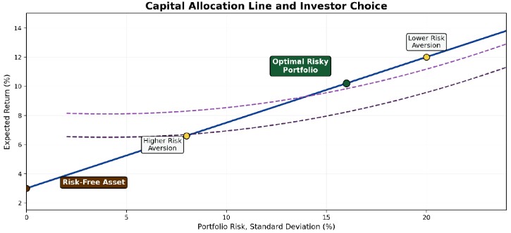
Figure 2 shows how investor preferences enter the decision. The CAL gives the attainable combinations of risk and return. A more risk-averse investor chooses a point closer to the risk-free asset. A less risk-averse investor chooses a point farther to the right and may even borrow at the risk-free rate to invest more than 100% in the risky portfolio. The optimal risky portfolio is common, but the final complete portfolio differs across investors.

Example 2: Choosing a Complete Portfolio on the CAL

Let’s say an investor can lend or borrow at a risk-free rate of 4.0% and invest in a diversified risky portfolio with an expected return of 11.0% and a standard deviation of 18.0%. The investor wants a complete portfolio with an expected return of 9.0%.

Find the risky-portfolio weight and the standard deviation of the complete portfolio.

Solution

Start by quoting the expected return formula:

$$E(r_c) = w_f r_f + (1 – w_f) E(r_Q)$$

It is often simpler to let \(y = 1 – w_f\), where \(y\) is the weight in the risky portfolio. Then:

$$E(r_c) = r_f + y [E(r_Q) – r_f]$$

Where:

• \(E(r_c) = 9.0\%\) is the target expected return of the complete portfolio
• \(r_f = 4.0\%\) is the risk-free rate
• \(E(r_Q) = 11.0\%\) is the expected return of the risky portfolio
• \(y\) is the weight invested in the risky portfolio

Solving for \(y\):

$$y = \frac{E(r_c) – r_f}{E(r_Q) – r_f}$$

$$y = \frac{9.0\% – 4.0\%}{11.0\% – 4.0\%} = 71.43\%$$

The risk-free weight is:

$$w_f = 1 – y = 28.57\%$$

Now quote the standard deviation formula:

$$\sigma_c = y \sigma_Q$$

Where:

• \(\sigma_c\) is the standard deviation of the complete portfolio
• \(y = 71.43\%\) is the weight invested in the risky portfolio
• \(\sigma_Q = 18.0\%\) is the standard deviation of the risky portfolio

Substitute the values:

$$\sigma_c = (0.7143)(18.0\%) = 12.86\%$$

The investor should allocate 71.43% to the risky portfolio and 28.57% to the risk-free asset. The complete portfolio’s standard deviation is 12.86%.

Example 3: Interpreting Leverage on the CAL

Imagine a second investor facing the same risk-free rate of 4.0% and the same risky portfolio with an expected return of 11.0% and standard deviation of 18.0%. This investor targets an expected return of 13.0%, which is higher than the risky portfolio’s expected return.

Again, use the formula:

$$y = \frac{E(r_c) – r_f}{E(r_Q) – r_f}$$

Where:

• \(E(r_c) = 13.0\%\) is the target expected return of the complete portfolio
• \(r_f = 4.0\%\) is the risk-free rate
• \(E(r_Q) = 11.0\%\) is the expected return of the risky portfolio
• \(y\) is the weight invested in the risky portfolio

Substitute the values:

$$y = \frac{13.0\% – 4.0\%}{11.0\% – 4.0\%} = 128.57\%$$

The risk-free weight is:

$$w_f = 1 – 1.2857 = -28.57\%$$

A negative risk-free weight means the investor borrows at the risk-free rate and invests more than 100% of wealth in the risky portfolio. The standard deviation is:

$$\sigma_c = (1.2857)(18.0\%) = 23.14\%$$

The investor’s target return is achievable only with leverage. This does not make the portfolio automatically inappropriate, but it does mean that the investor is taking materially more risk than the risky portfolio itself.

Selecting the Best Risky Portfolio

The investor’s final complete portfolio depends on risk aversion, but the best risky portfolio is the one that creates the steepest CAL. That is the risky portfolio with the highest Sharpe ratio.

$$ \textbf{Table 2: Comparing Candidate Risky Portfolios} \\
\begin{array}{l|c|c|c}
\textbf{Candidate Risky Portfolio} & \textbf{Expected Return} & \textbf{Standard Deviation} & \textbf{Sharpe Ratio at 3.0% Risk-Free Rate} \\
\hline
\text{Core Equity} & 9.0\% & 14.0\% & 0.43 \\ \hline
\text{Global Multi-Asset} & 11.0\% & 17.0\% & 0.47 \\ \hline
\text{Thematic Growth} & 13.0\% & 25.0\% & 0.40 \\
\end{array}
$$

Table 2 shows that the portfolio with the highest expected return is not necessarily the best risky portfolio. Thematic Growth has the highest expected return, but its volatility is also high. Global Multi-Asset provides the highest expected excess return per unit of risk and therefore creates the steepest CAL.

Example 4: Identifying the Risky Portfolio with the Highest CAL

Consider Table 2 above. Assume that the risk-free rate is 3.0%. Identify which risky portfolio an investor would use to build the best CAL.

Solution

Start with the Sharpe ratio formula:

$$\text{Sharpe Ratio} = \frac{E(r_Q) – r_f}{\sigma_Q}$$

Where:

• \(\text{Sharpe Ratio}\) is the slope of the CAL
• \(E(r_Q)\) is the expected return of the risky portfolio
• \(r_f = 3.0\%\) is the risk-free rate
• \(\sigma_Q\) is the standard deviation of the risky portfolio

For the Core Equity portfolio:

$$\frac{9.0\% – 3.0\%}{14.0\%} = 0.43$$

For the Global Multi-Asset portfolio:

$$\frac{11.0\% – 3.0\%}{17.0\%} = 0.47$$

For the Thematic Growth portfolio:

$$\frac{13.0\% – 3.0\%}{25.0\%} = 0.40$$

Global Multi-Asset has the highest Sharpe ratio. It creates the steepest CAL and is therefore the preferred risky portfolio under this framework. Investors with different risk aversion would combine that same risky portfolio with different amounts of the risk-free asset.

From CAL to CML

The capital market line, or CML, is a special case of the CAL. The CAL can be drawn using any risky portfolio. The CML is the line formed when the risky portfolio is the market portfolio.

The market portfolio is the portfolio of all risky assets, weighted by market value. In theory, it includes all investable risky assets, not just domestic equities. In practice, broad market indexes are often used as imperfect proxies.

The CML is:

$$E(r_c) = r_f + \frac{E(r_M) – r_f}{\sigma_M} \sigma_c$$

Where:

• \(E(r_c)\) is the expected return of a complete portfolio on the CML
• \(r_f\) is the risk-free rate
• \(E(r_M)\) is the expected return of the market portfolio
• \(\sigma_M\) is the standard deviation of the market portfolio
• \(\sigma_c\) is the standard deviation of the complete portfolio

The CML describes efficient complete portfolios formed from the risk-free asset and the market portfolio. More risk-averse investors hold more of the risk-free asset and less of the market portfolio. Less risk-averse investors hold more of the market portfolio and may use leverage.

Figure 3: From CAL to CML and CAPM

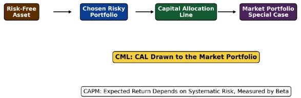
Figure 3 shows the progression. A CAL combines the risk-free asset with a chosen risky portfolio. When that chosen risky portfolio is the market portfolio, the line becomes the CML. CAPM then links an individual asset’s expected return to its contribution to market risk, measured by beta.

Example 5: Calculating Expected Return on the CML

Assume the risk-free rate is 3.0%, the expected return on the market portfolio is 10.5%, and the market portfolio’s standard deviation is 16.0%. An investor chooses a complete portfolio with a standard deviation of 10.0%.

Calculate the expected return implied by the CML.

Solution

We know that:

$$E(r_c) = r_f + \frac{E(r_M) – r_f}{\sigma_M} \sigma_c$$

Where:

• \(E(r_c)\) is the expected return of the complete portfolio
• \(r_f = 3.0\%\) is the risk-free rate
• \(E(r_M) = 10.5\%\) is the expected return of the market portfolio
• \(\sigma_M = 16.0\%\) is the standard deviation of the market portfolio
• \(\sigma_c = 10.0\%\) is the standard deviation of the complete portfolio

Substitute the values:

$$\begin{align*}
E(r_c) &= 3.0\% + \frac{10.5\% – 3.0\%}{16.0\%} (10.0\%) \\
E(r_c) &= 3.0\% + 4.6875\% = 7.69\%
\end{align*}$$

The complete portfolio’s expected return is 7.69%. The investor is holding a lower-risk position than the full market portfolio because the complete portfolio standard deviation is below the market portfolio’s standard deviation.

The Mutual Fund Theorem

The mutual fund theorem states that all investors can construct optimal portfolios using the same risky market portfolio and the risk-free asset. Investors differ only in how much they allocate to each.

This idea has a powerful implication. Under the assumptions of the model, investors do not need different risky portfolios to match different levels of risk aversion. They can hold the same market portfolio and adjust the risk level through borrowing or lending at the risk-free rate.

In practice, this theorem is an idealization. Investors face borrowing constraints, taxes, transaction costs, inflation needs, liquidity needs, and restrictions on certain assets. Still, the theorem is important because it separates two decisions: identify the best risky portfolio, and then choose how aggressively to combine it with the risk-free asset.

Beta and Systematic Risk

The CML applies to efficient complete portfolios. For individual securities, the relevant risk is not total standard deviation. The relevant risk is the security’s contribution to market risk. That contribution is measured by beta.

Beta can be calculated as:

$$\beta_i = \frac{\sigma_{i,M}}{\sigma_M^2}$$

Where:

• \(\beta_i\) is the beta of asset \(i\)
• \(\sigma_{i,M}\) is the covariance between asset \(i\) and the market portfolio
• \(\sigma_M^2\) is the variance of the market portfolio

It can also be expressed using correlation and standard deviations:

$$\beta_i = \rho_{i,M} \frac{\sigma_i}{\sigma_M}$$

Where:

• \(\rho_{i,M}\) is the correlation between asset \(i\) and the market portfolio
• \(\sigma_i\) is the standard deviation of asset \(i\)
• \(\sigma_M\) is the standard deviation of the market portfolio

A beta greater than 1 means the asset is more sensitive to market movements than the market portfolio. A beta less than 1 means the asset is less sensitive. A beta of 1 means the asset has market-level systematic risk.

CAPM and the Security Market Line

The capital asset pricing model, or CAPM, states that expected return depends on systematic risk as measured by beta:

$$E(r_i) = r_f + \beta_i [E(r_M) – r_f]$$

Where:

• \(E(r_i)\) is the expected return of asset \(i\)
• \(r_f\) is the risk-free rate
• \(\beta_i\) is the beta of asset \(i\)
• \(E(r_M)\) is the expected return of the market portfolio
• \(E(r_M) – r_f\) is the market risk premium

The security market line, or SML, plots expected return against beta. Assets with higher beta should have higher expected return, assuming the CAPM holds.

Figure 4: Security Market Line and Beta Sensitivity

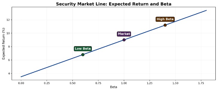
Figure 4 shows the core CAPM relationship. The risk-free asset has beta of zero. The market portfolio has beta of one. A higher-beta asset has a steeper exposure to the market risk premium and therefore requires a higher expected return.

Example 6: Estimating Beta and CAPM Expected Return

An analyst is estimating the required return on a listed semiconductor equipment company. The company’s return standard deviation is 24.0%, the market standard deviation is 16.0%, and the correlation between the company’s returns and market returns is 0.68. The risk‑free rate is 3.5%, and the expected market return is 9.0%.

Calculate the company’s beta and its expected return using CAPM.

Solution

Start with the beta formula:

$$\beta_i = \rho_{i,M} \frac{\sigma_i}{\sigma_M}$$

Where:

• \(\beta_i\) is the beta of the semiconductor equipment company
• \(\rho_{i,M} = 0.68\) is the correlation with the market portfolio
• \(\sigma_i = 24.0\%\) is the company’s return standard deviation
• \(\sigma_M = 16.0\%\) is the market portfolio’s standard deviation

Substitute the values:

$$\beta_i = 0.68 \times \frac{24.0\%}{16.0\%} = 1.02$$

Now use CAPM:

$$E(r_i) = r_f + \beta_i [E(r_M) – r_f]$$

Where:

• \(E(r_i)\) is the expected return of the company
• \(r_f = 3.5\%\) is the risk-free rate
• \(\beta_i = 1.02\) is the estimated beta
• \(E(r_M) = 9.0\%\) is the expected return on the market portfolio
• \(E(r_M) – r_f = 5.5\%\) is the market risk premium

Substitute the values:

$$E(r_i) = 3.5\% + 1.02(9.0\% – 3.5\%) = 9.11\%$$

The CAPM expected return is 9.11%. The result is driven by systematic risk. The company’s total volatility matters for beta only to the extent that the volatility is related to market movements.

Estimating Beta in Practice

Beta is commonly estimated by regressing an asset’s excess returns on market excess returns:

$$r_i – r_f = \alpha_i + \beta_i (r_M – r_f) + \epsilon_i$$

Where:

• \(r_i – r_f\) is the asset’s excess return
• \(r_M – r_f\) is the market portfolio’s excess return
• \(\alpha_i\) is the regression intercept
• \(\beta_i\) is the regression slope and estimated beta
• \(\epsilon_i\) is the regression error term

The slope coefficient is the beta estimate. The intercept, alpha, measures the average return not explained by the market excess return in the regression sample. Under a strict CAPM interpretation in an efficient market, expected alpha should be zero.

Beta estimates are sensitive to choices. Daily, weekly, or monthly returns can produce different estimates. A one-year sample may reflect current business conditions but be noisy. A five-year sample may be more stable but may miss recent changes in leverage, business mix, regulation, product exposure, or market structure. The market index used as a proxy also matters because the true market portfolio is not directly observable.

Limitations and Practical Judgment

The optimal-portfolio framework is elegant, but it rests on assumptions that do not always hold in practice. Returns may be skewed or fat-tailed, correlations may rise during stress, volatilities may shift across regimes, and expected returns are hard to estimate. Small estimation errors can produce surprisingly large changes in optimized weights.
Practical constraints also matter. Taxes, transaction costs, liquidity needs, borrowing limits, short-sale restrictions, benchmark mandates, and client-specific objectives can all move the final portfolio away from the clean theoretical result.

A disciplined analyst uses the model as a framework, not as a mechanical answer. The model clarifies the trade-off among expected return, risk, risk aversion, the risk-free asset, and systematic risk. The final portfolio still requires economic judgment.

Interpretation and Evaluation

Several practical principles follow:

• Risk-averse investors require higher expected return to bear additional risk.
• Utility increases with expected return and decreases with risk and risk aversion.
• The CAL shows combinations of a risk-free asset and a chosen risky portfolio.
• The slope of the CAL is the Sharpe ratio.
• The best risky portfolio is the one that produces the steepest CAL.
• More risk-averse investors choose lower-risk points on the CAL.
• Less risk-averse investors choose higher-risk points and may use leverage.
• The CML is the CAL formed using the market portfolio.
• Under CAPM, expected return depends on systematic risk, measured by beta.
• Beta is sensitive to the market proxy, return interval, and historical sample used in estimation.

Question

An investor can lend or borrow at a risk-free rate of 3.0%. The optimal risky portfolio has an expected return of 11.0% and a standard deviation of 16.0%. The investor wants a complete portfolio with an expected return of 9.0%.

The allocation to the risky portfolio and the complete portfolio’s standard deviation are closest to:

1. 50.0% and 8.0%
2. 75.0% and 12.0%
3. 112.5% and 18.0%

Answer Explanation

The correct answer is B.

Start by quoting the complete-portfolio expected return formula:

$$E(r_c) = r_f + y [E(r_Q) – r_f]$$

Where:

• \(E(r_c) = 9.0\%\) is the target expected return of the complete portfolio
• \(r_f = 3.0\%\) is the risk-free rate
• \(E(r_Q) = 11.0\%\) is the expected return of the optimal risky portfolio
• \(y\) is the allocation to the risky portfolio

Rearrange to solve for \(y\):

$$\begin{align*}
y &= \frac{E(r_c) – r_f}{E(r_Q) – r_f} \\
y &= \frac{9.0\% – 3.0\%}{11.0\% – 3.0\%} = 75.0\%
\end{align*}$$

Now  the standard deviation formula for a risk-free asset and a risky portfolio:

$$\sigma_c = y \sigma_Q$$

Where:

• \(\sigma_c\) is the standard deviation of the complete portfolio
• \(y = 75.0\%\) is the allocation to the risky portfolio
• \(\sigma_Q = 16.0\%\) is the standard deviation of the optimal risky portfolio

Substitute the values:

$$\sigma_c = (0.75)(16.0\%) = 12.0\%$$

The investor allocates 75.0% to the risky portfolio and 25.0% to the risk-free asset. The complete portfolio’s standard deviation is 12.0%.