What is the Central Limit Theorem in Finance?

Why Estimation Matters in Investment Analysis

Investment decisions are usually made with incomplete information. An analyst may observe five years of daily returns, several hundred trades, a sample of client accounts, or a limited number of fund managers. The true population parameter is normally unknown. The task is to use a sample statistic, such as a sample mean or sample standard deviation, to say something disciplined about the underlying population.

This learning outcome introduces the statistical foundation for that discipline. The central limit theorem explains why sample means can often be treated as approximately normally distributed when sample sizes are large. Confidence intervals convert a point estimate into a range that reflects sampling uncertainty. Sampling methodologies determine whether the sample is likely to support reliable inference in the first place.

The important exam idea is that calculation and interpretation are inseparable. A confidence interval is not just a formula. It is an estimate built on assumptions about data, sampling, and distributional behavior. If those assumptions are weak, the numerical result may look precise while being economically unreliable.

The Law of Large Numbers and the Central Limit Theorem

The law of large numbers says that, as the sample size increases, the sample mean tends to get closer to the population mean. This idea explains why larger samples usually produce more reliable estimates than smaller samples.

The central limit theorem, or CLT, goes further. It states that, if random samples are drawn from a population with a finite mean and finite variance, the sampling distribution of the sample mean becomes approximately normal as the sample size becomes large. This result can hold even when the original population is not normally distributed.

The expected value of the sample mean is:

$$E(\bar{X}) = \mu$$

Where:

• \(E(\bar{X})\) is the expected value of the sample mean
• \(\bar{X}\) is the sample mean
• \(\mu\) is the population mean

The variance of the sampling distribution of the sample mean is:

$$\sigma_{\bar{X}}^2 = \frac{\sigma^2}{n}$$

Where:

• \(\sigma_{\bar{X}}^2\) is the variance of the sampling distribution of the sample mean
• \(\sigma^2\) is the population variance
• \(n\) is the sample size

The standard deviation of the sample mean is called the standard error:

$$\sigma_{\bar{X}} = \frac{\sigma}{\sqrt{n}}$$

Where:

• \(\sigma_{\bar{X}}\) is the standard error of the sample mean
• \(\sigma\) is the population standard deviation
• \(n\) is the sample size

These formulas show why sample size matters. Doubling the sample size does not cut the standard error in half, because the standard error declines with the square root of the sample size. To reduce the standard error by half, the analyst needs roughly four times as many observations.

Visualizing the Central Limit Theorem

Figure 1: Central Limit Theorem and the Distribution of Sample Means

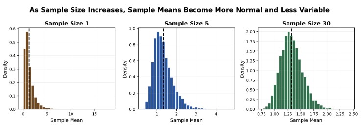
Figure 1 uses simulated observations from a right-skewed population. When the sample size is one, the distribution of observations remains skewed. When each sample mean is calculated from five observations, the sampling distribution begins to look more balanced. When each sample mean is calculated from thirty observations, the sampling distribution is tighter and more nearly normal. This is the practical force of the central limit theorem: large-sample averages are often more statistically manageable than individual observations.

The CLT is especially useful in finance because raw return data can be noisy, skewed, or influenced by occasional market shocks. It allows analysts to use normal-based confidence intervals and hypothesis tests for sample means when the sample is sufficiently large and the underlying assumptions are reasonable.

Standardizing the Sample Mean

The sample mean can be standardized using a Z-score:

$$Z = \frac{\bar{X} – \mu}{\sigma / \sqrt{n}}$$

Where:

• \(Z\) is the standardized value of the sample mean
• \(\bar{X}\) is the sample mean
• \(\mu\) is the hypothesized or true population mean
• \(\sigma\) is the population standard deviation
• \(n\) is the sample size

When the sample is large, this standardized value is approximately standard normally distributed:

$$Z \approx N(0, 1)$$

Where:

• \(N(0, 1)\) is the standard normal distribution
• \(0\) is the mean of the standard normal distribution
• \(1\) is the variance of the standard normal distribution

In practice, the population standard deviation is rarely known. Analysts often estimate it using the sample standard deviation, especially with large samples. The conceptual message does not change: the sample mean is compared with a reference value after being scaled by its sampling uncertainty.

Example 1: Applying the Central Limit Theorem to a Large Return Sample

An analyst has collected 225 weekly returns for a diversified digital infrastructure index. The sample mean return is 0.18% and the sample standard deviation is 3.60%. Estimate the standard error of the sample mean and interpret its meaning in the context of return precision.

Solution

We know that:

$$SE = \frac{s}{\sqrt{n}}$$

Where:

• \(SE\) is the estimated standard error of the sample mean
• \(s = 3.60\%\) is the sample standard deviation of weekly returns
• \(n = 225\) is the number of weekly return observations

Substituting the values:

$$SE = \frac{3.60\%}{\sqrt{225}} = \frac{3.60\%}{15} = 0.24\%$$

The standard error is 0.24%. This statistic measures the sampling uncertainty in the estimated mean, not the volatility of weekly returns themselves. The weekly returns vary with a standard deviation of 3.60%, but the estimated mean is much more precise because it is based on 225 observations.

Estimators and their Properties

A statistic used to estimate a population parameter is called an estimator. The sample mean is an estimator of the population mean. The quality of an estimator is judged by several properties.

An estimator is unbiased if its expected value equals the parameter it is intended to estimate:

$$E(\hat{\theta}) = \theta$$

Where:

• \(\hat{\theta}\) is an estimator of a population parameter
• \(\theta\) is the true population parameter
• \(E(\hat{\theta})\) is the expected value of the estimator

An estimator is consistent if it converges toward the true parameter as the sample size grows. A consistent estimate becomes more reliable as more relevant data become available.

An estimator is efficient if it has a smaller variance than alternative unbiased estimators. A minimum-variance unbiased estimator, or MVUE, is unbiased and has the lowest variance among all unbiased estimators. A best linear unbiased estimator, or BLUE, is the most efficient among unbiased estimators formed as linear combinations of the data.

A robust estimator is less sensitive to outliers, non-normality, and contaminated data. In finance, robustness matters because one crisis month, a bad data feed, or a structural break can distort ordinary averages.

$$ \textbf{Table 1: Properties of Estimators} \\
\begin{array}{l|c|c}
\textbf{Property} & \textbf{Meaning} & \textbf{Investment Interpretation} \\
\hline
\text{Unbiased} & {\text{Expected value equals the} \\ \text{parameter being estimated}} & {\text{The estimator is not systematically} \\ \text{too high or too low} }\\
\hline
\text{Efficient} & {\text{Lower variance among comparable} \\ \text{estimators}} & {\text{Estimates are more precise for a} \\ \text{given sample size}} \\
\hline
\text{Consistent} & {\text{Converges to the true parameter} \\ \text{as sample size increases}} & {\text{More relevant observations} \\ \text{improve reliability}} \\
\hline
\text{Robust} & {\text{Less affected by outliers or} \\ \text{non-normal data}} & {\text{Useful when financial data are} \\ \text{messy}}
\end{array} $$

Table 1 emphasizes that an estimator can be strong in one respect and weak in another. A mean may be unbiased for the population mean, but it may be less robust than a trimmed mean when the data contain extreme observations.

Confidence Intervals

A point estimate gives a single value, such as a sample mean of 0.18%. A confidence interval gives a range of plausible values for the unknown population parameter. The range is centered around the point estimate and widened by a margin of error.

For a large sample, the confidence interval for a population mean is:

$$\bar{X} \pm z_{\alpha/2} \frac{\sigma}{\sqrt{n}}$$

Where:

• \(\bar{X}\) is the sample mean
• \(z_{\alpha/2}\) is the critical value for a two-sided confidence interval
• \(\alpha\) is the total probability left outside the confidence interval
• \(\sigma\) is the population standard deviation
• \(n\) is the sample size

When the population standard deviation is unknown and the sample is large, the sample standard deviation is commonly used:

$$\bar{X} \pm z_{\alpha/2} \frac{s}{\sqrt{n}}$$

Where:

• \(s\) is the sample standard deviation
• all other terms are as previously defined

The margin of error is:

$$ME = z_{\alpha/2} \frac{s}{\sqrt{n}}$$

Where:

• \(ME\) is the margin of error
• \(z_{\alpha/2}\) is the two-tailed critical value
• \(s/\sqrt{n}\) is the estimated standard error

A 95% confidence interval does not mean there is a 95% probability that the fixed population mean lies inside the particular interval after it has been calculated. The population mean is fixed. The correct interpretation is procedural: if the analyst repeatedly drew samples in the same way and constructed intervals using the same method, about 95% of those intervals would contain the true population mean.

Figure 2: Confidence Interval Anatomy

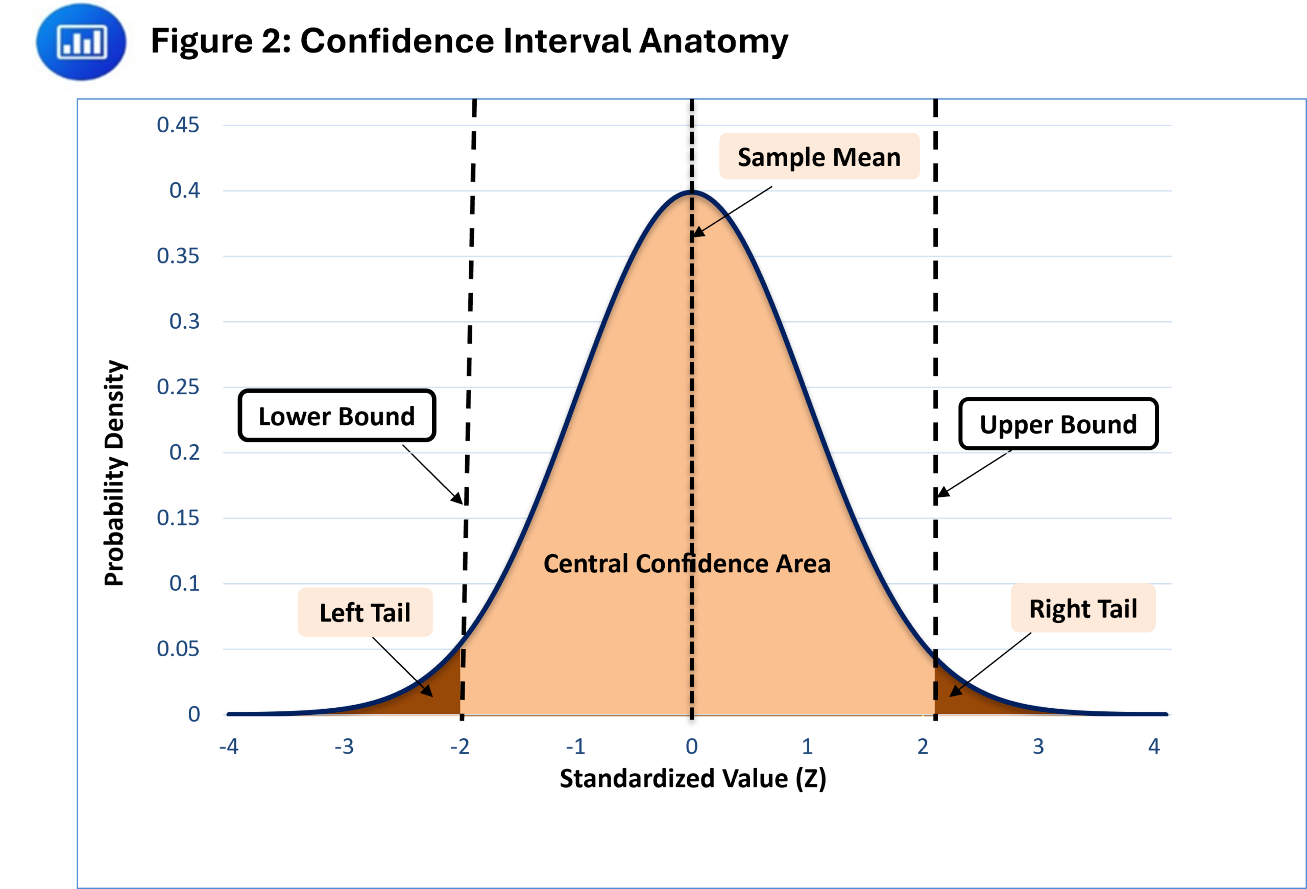
Figure 2 shows a two-sided confidence interval around a sample mean. The middle area represents the confidence level. The two tails together represent alpha, and each tail contains half of alpha. A higher confidence level moves the bounds farther from the sample mean, which produces a wider interval.

$$ \textbf{Table 2: Confidence Level, Tail Area, and Critical Value} \\
\begin{array}{c|c|c|c}
\textbf{Confidence Level} & \textbf{Total Tail Area} & {\textbf{Tail Area on} \\ \textbf{Each Side}} & { \textbf{Approximate} \\ \textbf{Z-Critical} \\ \textbf{Value}} \\
\hline
90\% & 10.0\% & 5.0\% & 1.645 \\ \hline
95\% & 5.0\% & 2.5\% & 1.960 \\ \hline
99\% & 1.0\% & 0.5\% & 2.576
\end{array}
$$

Table 2 shows why confidence intervals widen as confidence rises. A 99% interval needs to capture the true mean more often across repeated samples, so it uses a larger critical value than a 95% interval.

Example 2: Calculating 95% and 99% Confidence Intervals

Suppose an analyst is evaluating the average monthly excess return on an electric‑vehicle supply‑chain fund using 256 monthly observations. The sample mean return is 0.64%, and the sample standard deviation is 3.85%. Construct the 95% and 99% confidence intervals for the population mean monthly excess return and interpret the results.

Solution

Recall that:

$$\bar{X} \pm z_{\alpha/2} \frac{s}{\sqrt{n}}$$

Where:

• \(\bar{X} = 0.64\%\) is the sample mean monthly excess return
• \(s = 3.85\%\) is the sample standard deviation of monthly excess returns
• \(n = 256\) is the number of monthly observations
• \(z_{\alpha/2} = 1.960\) for a 95% two-sided confidence interval
• \(z_{\alpha/2} = 2.576\) for a 99% two-sided confidence interval

First calculate the standard error:

$$SE = \frac{3.85\%}{\sqrt{256}} = 0.2406\%$$

For the 95% confidence interval, the margin of error is:

$$ME_{95} = 1.960(0.2406\%) = 0.4716\%$$

The 95% confidence interval is:

$$0.64\% \pm 0.4716\% = [0.17\%, 1.11\%]$$

For the 99% confidence interval, the margin of error is:

$$ME_{99} = 2.576(0.2406\%) = 0.6198\%$$

The 99% confidence interval is:

$$0.64\% \pm 0.6198\% = [0.02\%, 1.26\%]$$

The 99% confidence interval is wider than the 95% confidence interval because it uses a larger critical value. The estimate is more conservative, but less precise.

What Makes Confidence Intervals Wider or Narrower?

The width of a confidence interval depends on three main inputs.

First, a higher confidence level increases the critical value and widens the interval. Second, a larger standard deviation increases the standard error and widens the interval. Third, a larger sample size reduces the standard error and narrows the interval.

$$ \textbf{Table 3: Drivers of Confidence Interval Width} \\
\begin{array}{l|l|l}
\textbf{Change} & \textbf{Effect on Confidence Interval Width} & \textbf{Reason} \\
\hline
\text{Higher confidence level} & \text{Wider} & \text{Larger critical value} \\
\hline
\text{Higher return volatility} & \text{Wider} & \text{Greater sampling uncertainty} \\
\hline
\text{Larger sample size} & \text{Narrower} & {\text{Standard error falls with the square} \\ \text{root of sample size}} \\
\hline
\text{Lower return volatility} & \text{Narrower} & \text{Lower sampling uncertainty} \\
\hline
\text{Lower confidence level} & \text{Narrower} & \text{Smaller critical value}
\end{array}
$$

Table 3 is an efficient way to answer many conceptual exam questions. A wider interval is not automatically better. It reflects greater confidence, more uncertainty, or both. A narrower interval is more precise, but it may be based on a lower confidence level or overly strong assumptions.

Confidence Intervals in Non-Stationary Financial Data

The central limit theorem requires a population with a finite mean and finite variance. In real financial datasets, those conditions may be strained. Asset prices can trend upward over long horizons. Volatility can change across regimes. Return distributions can show skewness, kurtosis, and crisis observations.

A confidence interval for the average return is usually more meaningful than a confidence interval for the average price of a trending asset. Percentage returns often remove much of the scale problem that affects price levels. Even then, the analyst should consider whether the return distribution has changed over time. A sample containing low-inflation years, high-inflation years, and crisis periods may not represent a single stable population.

The lesson is not that confidence intervals should be ignored. The lesson is that the interval should be interpreted with the data-generating process in mind.

Value at Risk as a One-Sided Confidence Interval

Value at risk, or VaR, uses confidence-interval logic to summarize downside risk. VaR answers a threshold question: how large a loss should not be exceeded with a chosen confidence level over a specified horizon?

A one-day VaR of USD 2 million at a 95% confidence level means there is a 5% probability that the portfolio loses more than USD 2 million in one day, assuming the model and inputs are correct. It does not mean the portfolio will lose exactly USD 2 million. It also does not describe how large losses may be beyond that threshold.

Figure 3: Value at Risk as a One-Sided Confidence Boundary

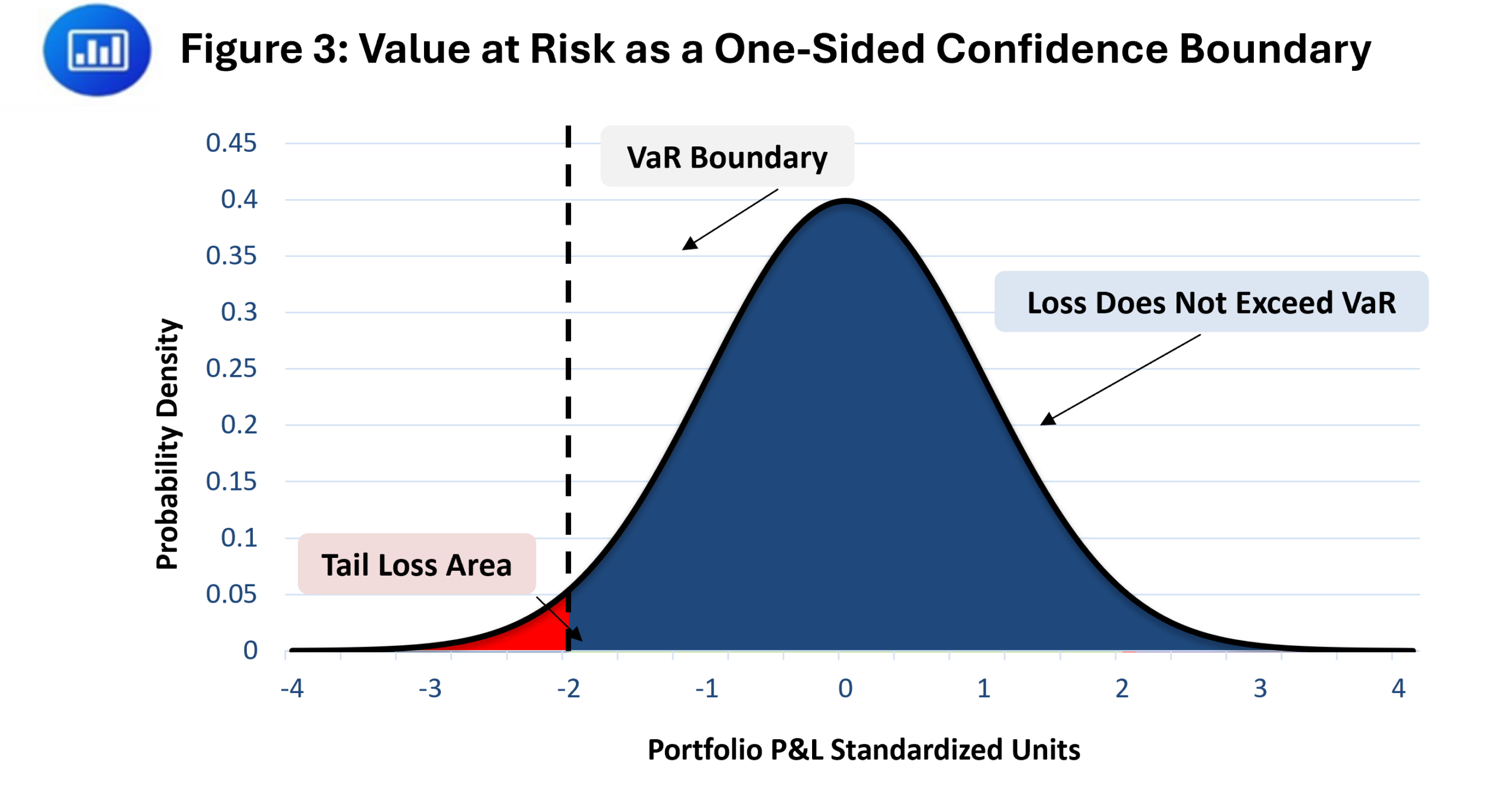
Figure 3 shows VaR as a left-tail boundary. The loss threshold is chosen so that only a specified tail probability lies beyond it. A 99% VaR leaves 1% in the left tail. VaR therefore focuses on downside risk and ignores upside outcomes.

Under a parametric variance-covariance approach with normally distributed returns and a zero expected return assumption, VaR can be estimated as:

$$VaR = z_c \sigma V$$

Where:

• \(VaR\) is the estimated loss threshold
• \(z_c\) is the one-sided standard normal critical value for confidence level \(c\)
• \(\sigma\) is the standard deviation of portfolio returns over the chosen horizon
• \(V\) is the current portfolio value

Parametric VaR is easy to calculate and communicate, but it has important limitations. It assumes that the chosen distribution and historical volatility are useful descriptions of future risk. It may understate tail risk when returns are skewed, fat-tailed, non-normal, or regime dependent. It also becomes less reliable for portfolios with nonlinear exposures such as options.

Example 3: Calculating Parametric VaR

Suppose we want to estimate the one-month 99% VaR for a CAD 25 million multi-asset portfolio. The analyst assumes normally distributed monthly returns, a zero expected monthly return, and a monthly standard deviation of 4.60%. The one-sided 99% standard normal critical value is 2.33.

Solution

We apply the formula:

$$VaR = z_c \sigma V$$

Where:

• \(z_c = 2.33\) is the one-sided 99% standard normal critical value
• \(\sigma = 4.60\% = 0.0460\) is the monthly standard deviation of portfolio returns
• \(V = \text{CAD } 25,000,000\) is the current portfolio value

Substitute the values:

$$VaR = 2.33(0.0460)(25,000,000) = \text{CAD } 2,679,500$$

The one-month 99% VaR is CAD 2.68 million. Under the model assumptions, there is a 1% probability that the portfolio loses more than CAD 2.68 million over one month. The estimate is model dependent and should not be interpreted as a worst-case loss.

Sampling Methodologies

Sampling determines whether statistical inference has a credible foundation. A carefully chosen sample can provide useful information about a population at much lower cost than observing every member. A poorly chosen sample can produce confidence intervals and test results that look rigorous but are biased from the start.

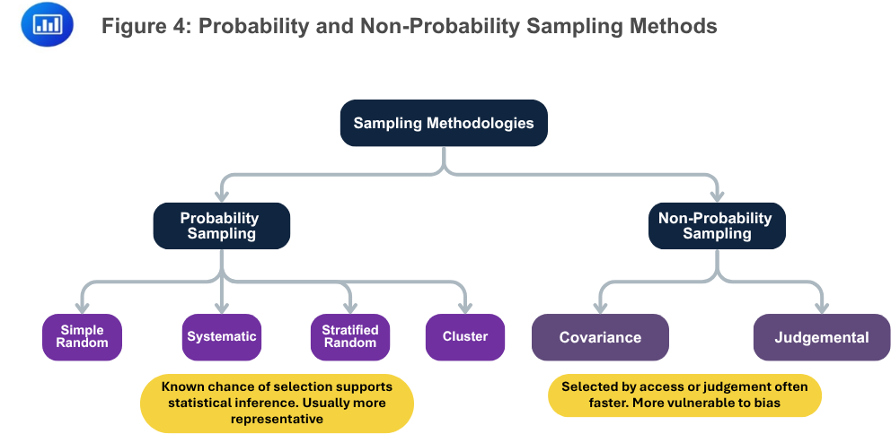
Figure 4 separates sampling methods into probability and non-probability approaches. Probability sampling gives population members a known chance of being selected and is generally more appropriate for statistical inference. Non-probability sampling may be useful for speed, expert review, or preliminary investigation, but it is more vulnerable to bias.

$$ \textbf{Table 4: Common Sampling Methods} \\
\begin{array}{l|c|c|c}
\textbf{Sampling Method} & \textbf{How It Works} & \textbf{Best Used When} & \textbf{Main Concern} \\
\hline
\text{Simple random sampling} & {\text{Each population element} \\ \text{has an equal chance of} \\ \text{selection}} & {\text{The population is fairly} \\ \text{homogeneous and a full} \\ \text{sampling frame exists}} & {\text{Random sampling error} \\ \text{and accidental imbalance}} \\
\hline
\text{Systematic sampling} & {\text{Every kth element is} \\ \text{selected after a starting} \\ \text{point}} & {\text{The list has no harmful}\\ \text{periodic pattern}} & {\text{Bias if the list order has a} \\ \text{pattern}} \\
\hline
{\text{Stratified random} \\ \text{sampling}} & {\text{Population is divided into} \\ \text{strata and random} \\ \text{samples are drawn within} \\ \text{each stratum}} & {\text{Important subgroups} \\ \text{must be represented}} & {\text{Requires accurate} \\ \text{stratum definitions}} \\
\hline
\text{Cluster sampling} & {\text{Population is divided into} \\ \text{clusters; selected clusters} \\ \text{are sampled}} & {\text{The population is} \\ \text{geographically or} \\ \text{operationally dispersed}} & {\text{Higher error if} \\ \text{observations inside} \\ \text{clusters are too similar}} \\
\hline
\text{Convenience sampling} & {\text{Easily available} \\ \text{observations are selected} }& {\text{Preliminary work or rapid} \\ \text{exploratory review}} & \text{Selection bias} \\
\hline
\text{Judgmental sampling} & {\text{Expert judgment} \\ \text{determines which} \\ \text{observations are selected} }& {\text{Targeted review, auditing,} \\ \text{specialist cases}} & \text{Subjective bias}
\end{array}
$$

Table 4 gives the practical interpretation of each method. Stratified random sampling is often attractive when important subgroups differ materially. Cluster sampling can reduce cost but may reduce precision when observations inside a cluster are highly similar. Convenience and judgmental sampling may be useful, but they do not usually justify the same statistical inference as probability samples.

Example 4: Selecting an Appropriate Sampling Method

Let’s assume the goal is to estimate the average transaction cost for institutional equity trades executed across three regions: North America, Europe, and Asia-Pacific. Trade size, market structure, and liquidity differ across the regions. The dataset is too large to review in full, but the analyst needs a representative estimate.

The best approach is stratified random sampling. The analyst should divide the population into regional strata and randomly select trades within each region, ideally in proportion to the region’s share of the full trade population or according to the precision needs of the study.

The objective is not merely to reduce the number of observations. The objective is to preserve representation of the groups that may have different transaction-cost behavior. A simple random sample might work if the sample is very large, but it could underrepresent a smaller region. A convenience sample of easily available trades would be faster but more vulnerable to bias.

Sampling Error and Sampling Distribution

Sampling error is the difference between a sample statistic and the population parameter it estimates. Sampling error arises because the sample is only a subset of the population.

Sampling error can be written generally as:

$$\text{Sampling Error} = \text{Sample Statistic} – \text{Population Parameter}$$

Where:

• \(\text{Sampling Error}\) is the estimation difference caused by using a sample
• \(\text{Sample Statistic}\) is the value calculated from the sample
• \(\text{Population Parameter}\) is the true value in the population

The sampling distribution of a statistic is the distribution of the statistic across all possible samples of the same size drawn from the same population. The CLT describes the sampling distribution of the sample mean under suitable conditions.

Example 5: Calculating Sampling Error

Assume we’d like to evaluate the sampling error in an estimate of average monthly client redemptions from a platform-based wealth manager. The true population mean redemption rate for the month is later found to be 1.40%, while the sample mean from the analyst’s survey is 1.55%.

Solution

We know that:

$$\text{Sampling Error} = \text{Sample Statistic} – \text{Population Parameter}$$

Where:

• \(\text{Sample Statistic} = 1.55\%\) is the sample mean redemption rate
• \(\text{Population Parameter} = 1.40\%\) is the population mean redemption rate
• \(\text{Sampling Error}\) is the difference between the sample estimate and the population value

Substituting the values:

$$\text{Sampling Error} = 1.55\% – 1.40\% = 0.15\%$$

The sample mean overstates the population mean by 0.15 percentage points. This error is not necessarily a mistake. It is the ordinary result of estimating a population value from a subset of observations.

Interpretation and Evaluation

Several practical principles follow:

• The CLT concerns the sampling distribution of the sample mean, not the distribution of the original population itself.
• The sample mean is an unbiased estimator of the population mean under appropriate sampling conditions.
• The standard error falls as sample size increases, but it falls with the square root of sample size.
• Confidence intervals combine a point estimate, a critical value, and a standard error.
• Higher confidence levels produce wider intervals.
• Larger samples and lower volatility produce narrower intervals.
• VaR is a one-sided confidence-interval concept focused on downside loss thresholds.
• Probability sampling is generally more reliable for statistical inference than non-probability sampling.
• Stratified random sampling can improve representation and precision when the population contains important subgroups.
• Sampling error is unavoidable when using samples, but a sound sampling design helps control it.

Question

An analyst studies 144 monthly returns for a thematic equity portfolio. The sample mean monthly return is 0.85%, and the sample standard deviation is 3.60%. The analyst wants a 95% confidence interval for the population mean monthly return using a large-sample normal approximation.

The 95% confidence interval is closest to:

1. \([0.26\%, 1.44\%]\)
2. \([0.36\%, 1.34\%]\)
3. \([0.56\%, 1.14\%]\)

The correct answer is A.

Recall the formula:

$$\bar{X} \pm z_{\alpha/2} \frac{s}{\sqrt{n}}$$

Where:

• \(\bar{X} = 0.85\%\) is the sample mean monthly return
• \(z_{\alpha/2} = 1.960\) is the 95% two-sided standard normal critical value
• \(s = 3.60\%\) is the sample standard deviation of monthly returns
• \(n = 144\) is the number of monthly observations

First calculate the standard error:

$$SE = \frac{3.60\%}{\sqrt{144}} = 0.30\%$$

Then calculate the margin of error:

$$ME = 1.960(0.30\%) = 0.588\%$$

The confidence interval is:

$$0.85\% \pm 0.588\% = [0.262\%, 1.438\%]$$

Rounded to two decimal places, the 95% confidence interval is [0.26%, 1.44%].