


Machine Learning: A Revolution in Risk ...
After completing this reading, you should be able to: Describe the machine learning... Read More

After completing this reading, you should be able to:
Constructing a portfolio requires several inputs. These include:
Portfolios are constructed based on specific constraints as agreed upon with a client. Such constraints may include not taking short positions and limiting the amount of cash in a portfolio. On the other hand, a portfolio manager can add its own constraints, e.g., making a portfolio neutral across economies and limiting individual stock positions to ensure diversification. Constraints make a portfolio less efficient because of the limited amount of securities to choose from.
Alternatively, a manager can replace a portfolio construction process, regardless of its complexity. A complicated portfolio construction procedure can be replaced with a direct unconstrained mean/variance optimization using an adjusted set of alphas and a suitable level of risk aversion. Alphas should be consistent with a manager’s goals and beliefs to simplify the implementation process.
If alphas are inconsistent with a manager’s expectations for the information ratio, they can rescale them.
A rough estimate for alpha can be obtained by the following equation:
$$ \text{alpha}=\text{volatility}\times\text{information coefficient (IC)}\times\text{score} $$
This way, the correlation between the expected return and the actual return is determined. Both the volatility and the IC are assumed to be constant. On the other hand, the score is assumed to follow a standard normal distribution. Therefore, alphas should have a standard normal distribution or a scale given by:
$$ \sigma \left( \alpha \right) \sim \text{ volatility }\times \text{ IC} $$
In this case, \(\sigma{\left({\alpha}\right)}\) is the standard deviation of alpha.
For example, a 0.20 IC and typical volatility of 30% leads to an alpha scale of 6%. In this case, the alphas will have a mean of 0 and a standard deviation of 6%.
Including a constraint decreases the scale of alphas resulting in a decrease in the information coefficient. If the alphas’ input to portfolio construction does not have the proper scale, then they need to be rescaled.
Alphas can also be refined by trimming outliers. This is done by reducing extreme positive or negative alphas. In this context, extreme refers to all stocks that are greater in magnitude than three times the scale of alphas.
Trimming also involves forcing the alphas to be normally distributed, having a benchmark alpha of zero, and the required scale factor. Since the alpha typically utilizes the ranking information in the alphas while ignoring the alphas’ sizes, such an approach is extreme. The neutrality and scaling of the benchmark must be rechecked after such a transformation.
Neutralization is the process of removing biases or undesirable bets from alphas. Its implications are usually in terms of alphas and portfolios. The following are methods of refining alphas to be neutral.
Benchmark neutralization involves making the alphas of the benchmark zero. This is achieved by matching the beta of the benchmark portfolio to the beta of the active portfolio. A benchmark alpha of 0 ensures that the alphas are benchmark-neutral and eliminates benchmark timing.
If the benchmark has non-zero alphas, the neutralization process rescales the alphas to eliminate the benchmark alpha.
The following transformation guarantee that the benchmark will have zero alpha
$$ \begin{align*} \alpha_{Modified} = &\alpha-\alpha_{\beta}\times\beta \\ \\ \text{Modified benchmark neutral alpha} = &\text{Active position alpha} \\ & – \text{(Benchmark alpha × Active position Beta)} \end{align*} $$
Given the following:
$$ \begin{array}{l|c} {} & \textbf{Value} \\ \hline \text{Active position alpha} & {0.6\%} \\ \hline \text{Active position Beta} & {1.6} \\ \hline \text{Benchmark alpha} & {0.016\%} \end{array} $$
The modified benchmark neutral alpha can be calculated as:
$$\text {Neutral alpha}= 0.6-\left({1.6}\times{0.016}\right)=0.5744 $$
Benchmark neutralization implies that the optimal portfolio will have a beta of 1 from the portfolio perspective. For example, if a portfolio’s modified alpha has a Beta factor of 1.3, then this value can be adjusted to 1 by making the alpha benchmark neutral.
Alphas of a portfolio can also be made cash neutral. This is done by modifying alphas to eliminate any active cash position. Alphas can be made both cash and benchmark neutral.
Returns can be separated along various dimensions using the multiple-factor approach of portfolio analysis. Each of these dimensions can either be viewed as a source of risk or a source of active return.
In line with this definition, a manager cannot estimate risk factors. Therefore, he or she should neutralize the alphas against such risk factors. This is to say that a manager must neutralize the factors for which they do not have adequate information. Neutralized alphas of these risk factors will be zero.
Transaction cost is the cost incurred when changing from one position to another. Besides complicating the portfolio construction problem, transaction costs force greater precision in the choice of scale and the estimated alphas. Note that precision in scale is essential in addressing the tradeoff between alphas and transaction costs.
Maximization of risk-adjusted annual active return is the goal of portfolio construction. This requires a rebalancing of the portfolio, which attracts transaction costs. A rule to allocate the transaction costs is required to contrast transaction costs incurred at that time with alphas and active risk expected. Transaction costs must be amortized to make a comparison of the gain rate per year derived from the alpha and the annual rate of loss arising from active risk.
Consider two stocks. Of the two, the price of one will increase from $1.00 to $1.05 over six months. This stock can be replaced by another stock with a current price of $1.00, which will increase to $1.10 over the next year. The transaction cost is 2%. The annual alpha for both stocks is 3%.
The annual returns on the first stock will be approximately \((5\% – 2\%)×2 = 6\%\) and the annual returns on the second stock will be approximately \((10\% − 2\%) = 8\%\).
The holding period across portfolios is uncertain. Therefore, there is a question of the period over which to amortize the transaction costs. Typically, the annual transaction cost is the round-trip cost divided by the holding period in years. Notice that for the first stock, the holding period is 6 months. We have doubled the round-trip transaction cost to get the cost of the annual transactions.
An optimality relationship can be obtained between the information ratio, the risk aversion, and the optimal active risk. Since the information ratio and desired level of active risk are known, an appropriate risk aversion can be determined using the following equation:
$$ { \lambda }_{ \text{A} }=\cfrac { \text{IR} }{ { 2\sigma }_{ \text{p} } } $$
Where:
\({ \lambda }_{A}\) is the risk aversion.
\({ \text{IR} }\) is the information ratio.
\({ \sigma }_{ \text{p} }\) is the active risk.
A portfolio has an information ratio of 50% and an acceptable level of volatility of the active return of 8%.
Calculate the implied risk aversion of the portfolio.
$$ \begin{align*} { \lambda }_{ \text{A} }&=\cfrac { \text{IR} }{ { 2\sigma }_{ \text{p} } } \\ &=\cfrac {50\%} {2 \times 8\%}=3.125 \end{align*} $$
Note: We must be careful that our optimizer is using percentages and not decimals.
Determining the aversion to specific rather than common-factor risk utilizes a different approach. The following decomposition of risk is utilized by several commercial optimizers to allow differing aversions to different sources of risk:
$$ \text{U}={ \alpha }_{ \text{p} }-\left( { \lambda }_{ \text{A,CF} }{ \sigma }_{ \text{p,CF} }^{ 2 }+{ \lambda }_{ \text{A,SP} }{ \sigma }_{ \text{p,SP} }^{ 2 } \right) $$
Where:
\({\alpha}_{ \text{p} }\) is the portfolio alpha.
\({\sigma}_{ \text{p} }\) is the active risk.
\({ \lambda }_{ \text{A} }\) is the risk aversion.
The two reasons for considering the implementation of a higher risk aversion to specific risk include:
A benchmark with a weight of zero can be expanded to include forecasted stocks that are not in the benchmark. This keeps stock n in the benchmark, which has zero weight in determining the benchmark return or risk.
Stocks without forecast returns in the benchmark can be dealt with by employing the following approach:
Assume that the collection of stocks with forecasts is represented by \({ \text{N} }_{1}\) and the stocks without forecasts by \({ \text{N} }_{0}\). The value-weighted fraction of stocks with forecasts will be the sum of active holdings with forecasts:
$$ \text{H}\left\{ { \text{N} }_{ 1 } \right\} =\sum _{ \text{n}\in { \text{N} }_{ 1 } }^{ }{ { \text{h} }_{ \text{B,n} } } $$
The average alpha for the stocks with forecasts, group \({ \text{N} }_{1}\), is
$$ { \alpha }\left\{ { \text{N} }_{ 1 } \right\}= \cfrac{ \text{Weighted average of alphas with forecasts} } {\text{Value-weighted fraction of stocks with forecasts} } =\cfrac { \sum _{ { { \text n }\in { { \text N } }_{ 1 } } }{ } {\text h }_{ \text B,{\text n} }{ \alpha }_{\text n }}{ \text{H}\left\{ { \text{N} }_{ 1 } \right\} } $$
We set \( { \alpha }_{ \text{n} }^{ * }={ \alpha }_{ \text{n} }-\alpha \left\{{ \text{N} }_{1} \right\} \) to round out the set of forecasts for the stock in \({ \text{N} }_{1}\) and an \( { \alpha }_{ \text{n} }^{ * }=0 \) for stocks in \({ \text{N} }_{0}\) . These alphas are benchmark-neutral. Additionally, the stocks we did not cover will have a zero, and therefore neutral, forecast.
A portfolio should be revised when new information is received. Frequent revisions are not a challenge to a manager with the skills to make a correct tradeoff between expected active return, transaction costs, and active risks.
A manager who underestimates transaction costs will have to trade more frequently. Frequent trading causes a great deal of uncertainty in the alpha estimates. A manager should, therefore, revise the portfolio less frequently to avoid incurring transaction costs higher than expected, with lower-than-expected alphas.
Decreasing the time horizon of the expected alphas increases their amount of noise despite the actual transaction costs estimates. Noisier returns are witnessed with shorter horizons. Therefore, frequent reactions to noise rather than signal would be involved in rebalancing for very short horizons.
Due to the inherent importance of the time horizon, it becomes difficult to analyze the tradeoff between alpha, risk, and costs. However, we can capture the value of new information and decide whether to trade by comparing the marginal contribution to value-added for a given stock n, \({ \text{MCVA} }_{ \text{n} }\), to the transaction costs.
$$ { \text{MCVA} }_{ \text{n} } = { \alpha }_{ \text{n} } -2 \times { \lambda }_{ \text{A} } \times \sigma \times { \text{MCAR} }_{ \text{n} } $$
Where:
\({ \alpha }_{\text{n}}\) is the alpha of asset n.
\({ \lambda }_{ \text{A} }\) is the risk aversion.
\({ \sigma }\) is the active risk.
\({ \text{MCAR} }_{ \text{n} }\) is the marginal contribution to the active risk of asset.
The marginal contribution to the value-added of a newly purchased stock is equal to its purchase cost. A no-trade region exists when the benefits of rebalancing are less than the costs. In other words, a no-trade region emerges when the negative cost of selling is less than the purchase cost. That is:
$$ \text{- selling cost < marginal contribution to value-added < } \text {cost of purchase} $$
Mathematically expressed as:
$$ -{ \text{SC} }_{ \text{n} }\le { \text{MCVA} }_{ \text{n} } \le { \text{PC} }_{ \text{n} } $$
or
$$ {2 \lambda}_{ \text{A} } \sigma{ \text{MCAR} }_{ \text{n} }-{ \text{SC} }_{ \text{n} }≤{ \alpha }_{ \text{n} }≤{ \text{PC} }_{ \text{n} }+{2 \lambda}_{ \text{A } } \sigma{ \text{MCAR} }_{ \text{n} } $$
Knowing when to rebalance calls for the analysis of the dynamic problem involving alphas, risks, and costs over time.
The following four procedures cover the vast majority of institutional portfolio management applications:
Since a manager’s interest is high alpha, low active risk, and low costs of transactions, value-added minus the costs of transactions is the figure of merit:
$$ \text{Manager’s value}=\alpha_{ \text{P} }-{ \lambda }_{ \text{A} } { \sigma }_{ \text{P} }^{2}-{ \text{TC} } $$
Where:
\( { \alpha }_{ \text{P} } \) is the portfolio alpha.
\( { \lambda }_{ \text{A} } \) is the risk aversion.
\( { \sigma }_{ \text{P} }^{2} \) is active risk squared.
\( \text{TC} \) is the transaction cost.
Stock screens are used by equity investment managers to rank stocks according to a given criterion to identify desirable and undesirable investments. For instance, if an investment manager believes that a low price-to-earnings ratio (P/E) indicates a company’s hidden value, they may use P/E to rank companies in the investment world.
Stratification eliminates sample bias by dividing the total population into distinct sub-populations (samples), which are representative of the whole population. The list of stocks is split into exclusive categories. Stock screens are then executed within the individual categories to construct a portfolio. Alpha is used to rank the stocks and place them into the buy, hold, and sell list within the categories keeping a reasonable turnover. The stocks are then weighted to ensure that the portfolio weight matches the benchmark weight in that category.
Stratification is an improvement in screening and, therefore, has the same benefits as stock screening.
A linear program (LP) uses risk dimensions such as volatility, beta, and size, among others, to put stocks into categories. Unlike stratification, these categories do not need to be exclusive. The linear program then constructs an optimal portfolio. This is done by maximizing the portfolio’s alpha minus transaction costs while remaining close to the benchmark portfolio in the risk control dimensions.
Quadratic programming includes alpha, risk, and transaction costs. Moreover, a quadratic program can include all the constraints and limitations encountered in a linear program. The constraints are linear while the objective function is quadratic.
Estimation errors within 1% do not have a significant impact on the value-added. However, as the estimation error increases (underestimating volatility, by say, 5%, below the actual volatility), the value-added becomes negative. Note that estimation errors lead to inefficient estimation. Moreover, it is vital to have reasonable estimates of covariance.
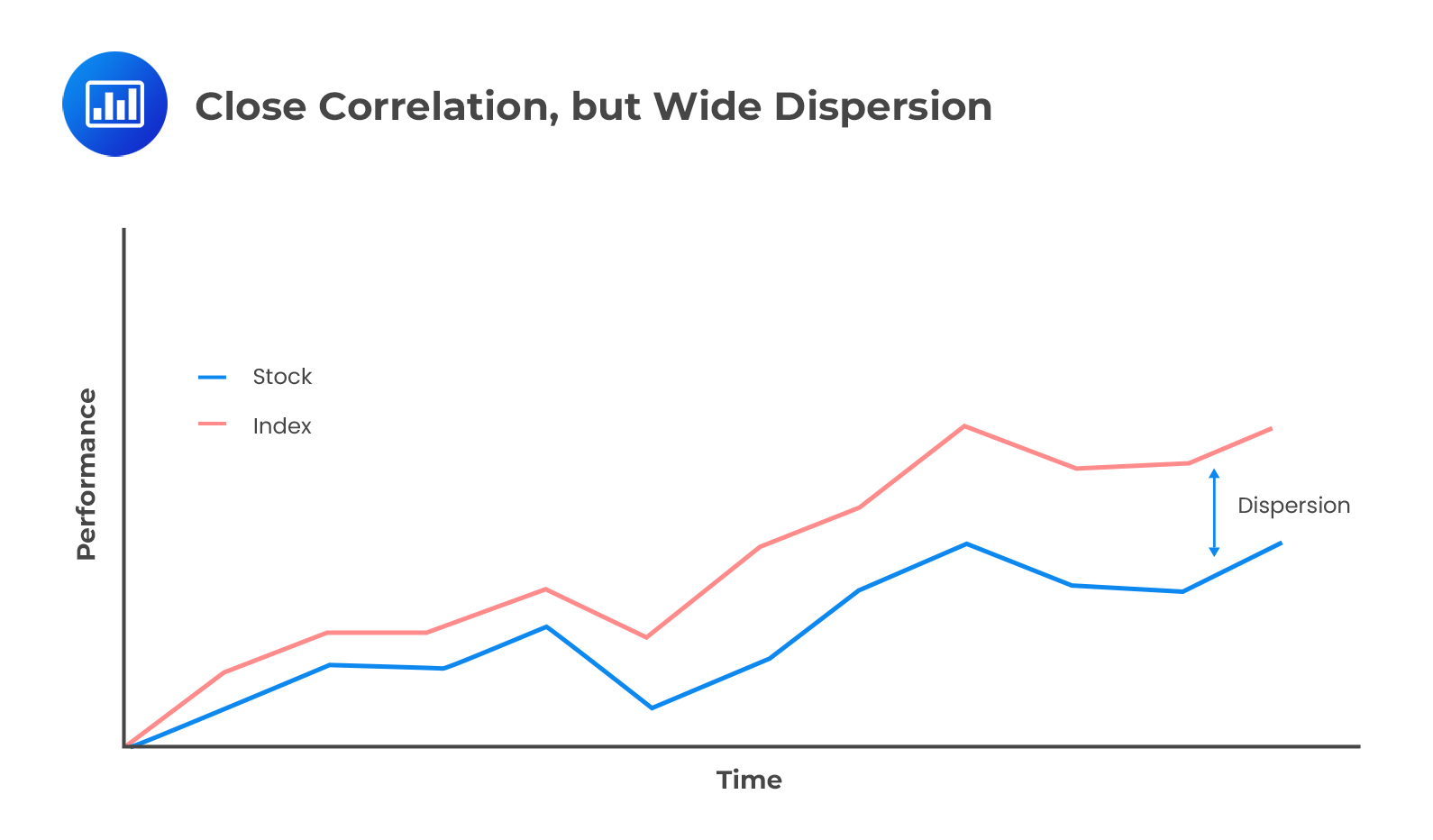
Dispersion is the range of possible returns on investment. In other words, it is the difference between the minimum and maximum returns of the separate portfolios. The dispersion of return on investment shows the volatility and risk of holding it.
A more variable return on a given asset implies more risk or volatility. For instance, if an asset’s historical return in a given year is in the range of +10% to -10%, then it is more volatile since there is a wide dispersion of returns than one whose historical return is in the range of +3% to -3%. The higher the dispersion, the higher the potential of gaining meaningful returns above the average return of the index.
The following figure illustrates the dispersion.
 Sources of Dispersion
Returns vary across client accounts. This is because clients impose different constraints leading to different portfolios. These different constraints initiated by clients lead to dispersion, which is beyond a manager’s control.
A manager’s lack of attention gives rise to different accounts exhibiting different betas and different factor exposures. Managers can reduce this form of dispersion through proper supervision and control.
Having identical client accounts would ensure that there is no dispersion. However, this is impossible, given transaction costs. Nonetheless, managers can achieve zero-dispersion with increased transaction costs. For a given amount of transaction costs, there is an optimal level of dispersion that balances gains from portfolio rebalancing transaction costs. Dispersion should be reduced to an extent where further reduction would substantially decrease average returns due to the incurrence of higher transaction costs.
The convergence of dispersion depends on the type of alphas, the transaction costs, and the portfolio construction methodology. If alphas and active risk do not change over time, dispersion will never disappear due to the transaction cost barrier. The exact matching of portfolios will also never pay. Furthermore, the remaining active risk is bounded based on the transaction costs and the manager’s risk aversion.
Very high-risk aversion implies that all portfolios must be close to one another. The higher the transaction costs, the higher the active risk. Dispersion is proportional to active risk. The constant of proportionality depends on the number of managed portfolios.
With the active risk constant, increasing the number of managed portfolios increases the dispersion as more portfolios explore the extremes of the return distribution.
Convergence occurs if alphas and risk vary over time. This is because the portfolios will either maintain or, more typically, decrease the amount of dispersion. Ultimately, this will lead to the convergence of returns. However, the rate at which convergence will occur is uncertain.
Convergence can be increased by changing the portfolio construction technology. Mainly, dual-benchmark optimization can reduce dispersion, but only at an undesirable price. Dual-benchmark optimization simply introduces the tradeoff between dispersion and return.
Practice Question
Margaret is the lead portfolio manager at Phoenix Investment Group, a boutique firm known for its active management style. Recently, she took a deep dive into her active portfolio, which consists of various assets spread across different industries. She noticed that despite the robust alpha generation in the portfolio, it seems to be significantly affected by unintended bets and biases. After a thorough discussion with her team, Margaret decided that it was crucial to refine the alphas and neutralize certain biases. Her goal is to minimize these unintended bets while maintaining the portfolio’s active strategy.
Based on the scenario presented, which approach should Margaret adopt to refine the alphas in her portfolio and achieve her goal?
A. Adjust alphas to remove any unintended bets on small-cap versus large-cap returns. B. Modify alphas only to account for the difference in market returns between her active portfolio and the benchmark.
C. Adjust alphas to ensure that her active portfolio has an identical beta to that of the benchmark.
D.Neutralize industry risk factors only by subtracting the average alpha for an industry from the alphas of each firm within that industry.
Solution
The correct answer is C.
Margaret aims to minimize unintended bets and biases in her portfolio. One of the most comprehensive ways to achieve this is through benchmark neutralization. As the study notes suggest, benchmark neutralization eliminates any difference between the benchmark beta and the beta of the active portfolio. In essence, by adjusting the alphas so that the active portfolio’s beta matches the benchmark’s beta, Margaret can ensure that her portfolio remains neutral to most unintended market bets, thereby achieving her primary goal.
A is incorrect. While adjusting alphas to remove unintended bets on small-cap versus large-cap returns is a valid method, it only addresses one specific risk factor. Margaret’s concern, as described in the vignette, is more holistic, making this approach insufficient for her broader goal.
B is incorrect. Modifying alphas to account for market return differences only captures a portion of the biases. While market returns play a role in portfolio performance, they are just one of many factors. To truly neutralize biases, Margaret would need to look beyond just market return differences.
D is incorrect. Neutralizing only industry risk factors might address biases within specific sectors, but it doesn’t comprehensively tackle other potential market or risk-factor biases present in the portfolio. Margaret’s goal is to minimize a wide range of unintended bets, not just those related to industries.
Things to Remember
- Benchmark neutralization aligns the active portfolio’s beta with the benchmark’s beta, neutralizing unintended market bets.
- Refining alphas requires a comprehensive strategy, not just addressing isolated risk factors.
- The goal of refining alphas is to retain an active strategy while minimizing unintended exposures.
Offered by AnalystPrep


