


Foreign Exchange Markets
After completing this reading, you should be able to: Explain and describe the... Read More
After completing this reading, you should be able to:
Constant volatility is easily approximated from historical data. However, volatility varies through time. Therefore, an alternative to constant normality of asset returns is to assume that asset returns are normally distributed conditioned on a known volatility. More specifically, high volatility indicates that the daily asset return is normally distributed with high standard deviation, and when the volatility is low, the daily returns are normally distributed with low standard deviation.
Monitoring volatility is made possible through two methodologies (as will be covered later in this chapter): the exponentially weighted moving average (EMWA) model and he GARCH (1,1) model. We will also apply the estimation of the volatility and application of volatility monitoring to correlation.
There are several reasons as to why the normality framework has been adopted in most risk estimation attempts. For starters, a normal distribution is relatively easy to implement. We need two parameters – the mean, \({ \mu }\), and the standard deviation, σ, of returns. With these two, it is possible to characterize the distribution fully and even come up with Value at Risk measures at specified levels of confidence. In the real world, however, asset returns are not normally distributed, and this can be observed empirically. Asset return distributions exhibit several attributes of non-normality. These are:
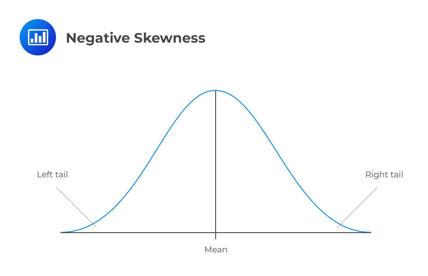
For this reading, it’s essential to keep in mind that the term ‘fat tails’ is relative: it refers to the tails of one distribution relative to normal distribution. If a distribution has fatter tails relative to the normal distribution, it has a similar mean and variance, but probabilities at the extremes are significantly different.
When modeling asset returns, analysts focus on extreme events – those that have a low probability of occurrence but result in catastrophic losses. There’s no point concentrating on non-extreme events that ordinarily aren’t expected to cause severe losses.
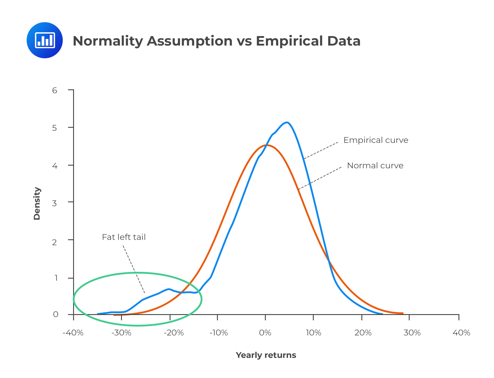
If we were to assume that the normal distribution holds as far as asset returns are concerned, we would not expect even a single daily move of 4 standard deviations or more per year. The normal distribution predicts that about 99.7% of outcomes lie within 3 standard deviations from the mean.
In reality, every financial market experience one or more daily price moves of 4 standard deviations or more every year. There’s at least one market that experiences a daily price move of 10 or more standard deviations per year. What then does this suggest?
The overriding argument is that the true distribution of asset returns has fatter tails.
There is a higher probability of extreme events than the normal distribution would suggest. This means that reliance on normality results in inaccurately low estimates of VaR. As a result, firms tend to be unprepared for such tumultuous events and are consequently heavily affected, sometimes leading to foreclosure and/or large-scale ripple effects that reverberate and destabilize the entire financial system.
Unconditional normal distribution manifests when the mean and standard deviation of asset returns in a model is the same for any given day, regardless of market and economic conditions. In other words, even if there is information about the distribution of asset returns that suggests the existence of different parameters, we ignore that information and assume that the same distribution exists on any given day.
Conditionally normal distribution occurs when a model contains asset returns that are normal every day, but the standard deviation of the returns varies over time. That is the standard deviation high at times and low at some other times.
The underpinning idea here is that if we collect daily return data, we will observe the unconditional distribution. Further, by monitoring volatility, we can estimate the conditional distribution for daily return. For instance, consider that from the (historical) data we have collected, we estimate volatility to be 0.5% per day. However, from volatility monitoring, we estimate the volatility to be 1.5% per day. Therefore, it will be more accurate to assume that asset returns are normally distributed with a 1.5% standard deviation. Thanks to this assumption, we use this 1.5% measure to calculate VaR and the Expected Shortfall (ES). In other words, it’s more advisable to use results from monitoring volatility than results from the fat-tailed distribution. Further, note that it is inadvisable assume a normal distribution with volatility from the observed data.
In an attempt to model asset returns better, analysts may subdivide a specified time period into regimes. In such an instance, each regime has a clearly noticeable set of parameters that are distinctly different from those of other regimes. For example, volatility could rise sharply during a market crash only to stabilize when conditions improve. This is the idea behind the regime-switching volatility model.
For illustration, let us use the real interest rates of a developed nation between 1990 and 2015:
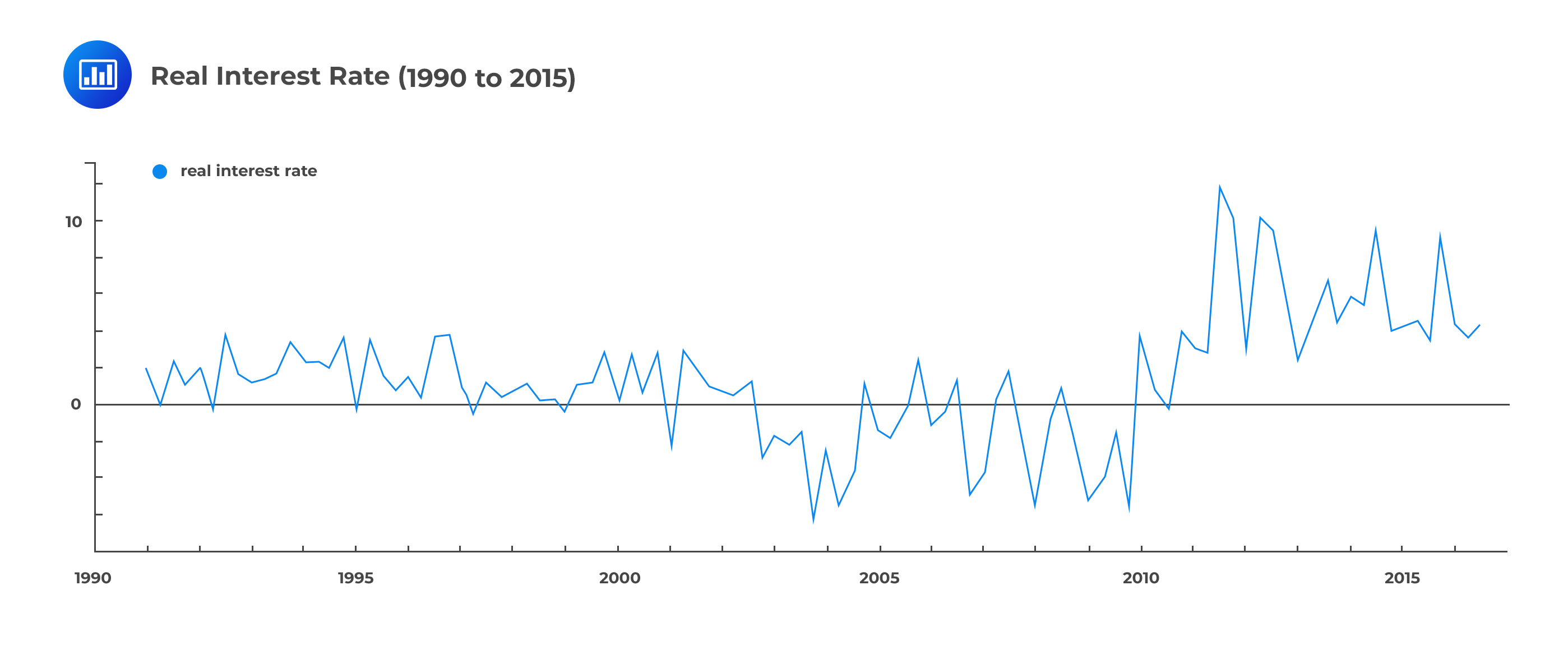 Given the graph above, it would be difficult to identify different states of the economy. Now, suppose we make use of an econometric model to try and identify the different economic states.
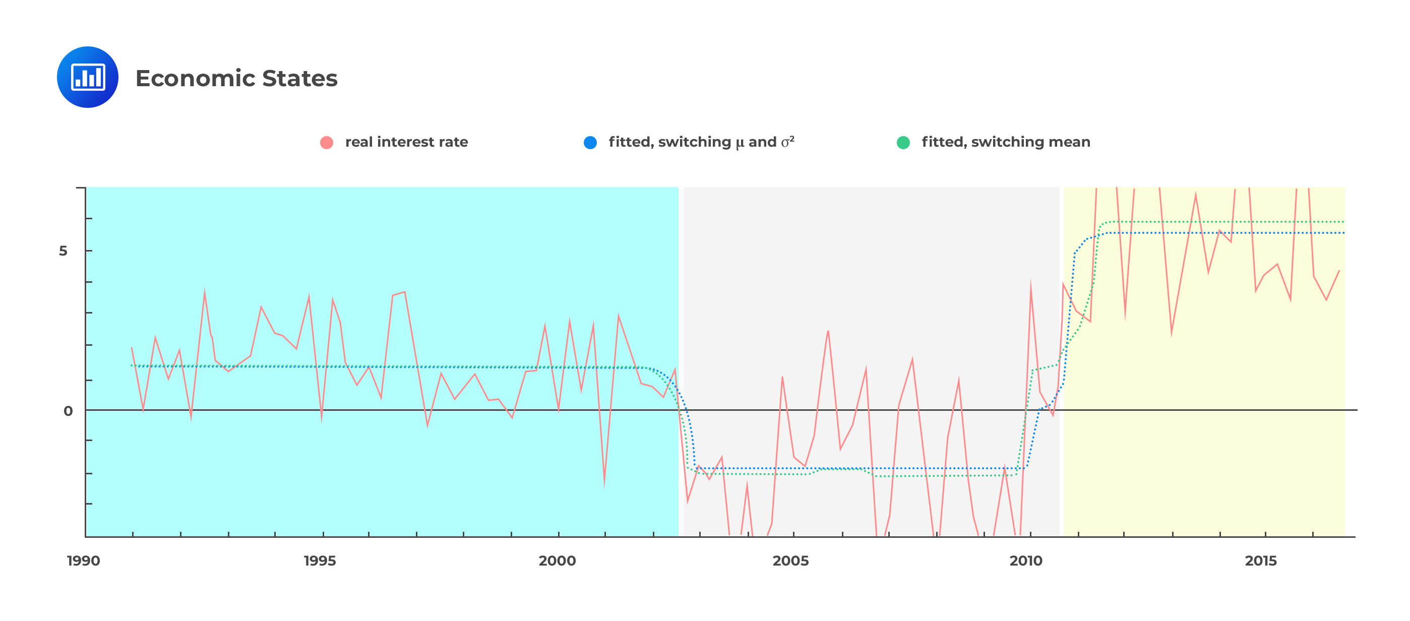 From the econometric model above, we can identify three distinct states of the economy. These are precisely what we would call regimes. As we switch from one regime to another, at least one parameter has to change. So, how exactly does the regime-switching model help to better measure volatility?
The conditional distribution of returns is always normal with either low or high volatility but a constant mean. The regime-switching model captures the conditional normality and, in so doing, helps resolve the fat tails problem.
Conventionally volatility is defined as a change of a variable value over a period of time. In the context risk management, volatility is defined as the standard deviation of an asset return in one day.
The assets return in a day i is defined as:
$$ \text{r}_{\text{i}}=\cfrac{{ \text{S} }_{ \text{i} }-{ \text{S} }_{\text{i}-1}}{\text{S}_{\text{i}-1} } $$
Where:
\(\text{r}_{\text{i}}\): Return on a day i.
\({ \text{S} }_{ \text{i} }\): Value of an asset on a close of trading i.
\({\text{S}_{\text{i}-1} }\): Value of an asset on a close of trading i-1.
For a day n, the variance \(({\sigma}_{\text{n}}^{2} )\) from the previous m days is given by
$$ { \sigma }_{ \text{n} }^{ 2 }=\cfrac { 1 }{ \text{m}-1 } \sum _{ \text{i}=1 }^{ \text{m} }{ { \left( { \text{r} }_{ \text{n}-\text{i} }-\bar { \text{r} } \right) }^{ 2 } } $$
And thus the standard deviation is given by:
$$ { \sigma }_{ \text{n} }=\sqrt{\left(\cfrac { 1 }{ \text{m}-1 } \sum _{ \text{i}=1 }^{ \text{m} }{ { \left( { \text{r} }_{ \text{n}-\text{i} }-\bar{ \text{r} } \right) }^{ 2 } }\right)} $$
Where:
\(\bar{ \text{r} }\): average return from the previous m-days defined as:
$$ \bar { \text{r} } =\cfrac { 1 }{ \text{m} } \sum _{ \text{i}=1 }^{ \text{m} }{ { \text{r} }_{ \text{n}-\text{i} } } $$
The risk management simplifies the above formulas by:
Therefore, defining the variables as before, the formula for the standard deviation changes to:
$$ { \sigma }_{ \text{n} }^{ 2 } =\cfrac { 1 }{ \text{m} } \sum _{ \text{i}=1 }^{ \text{m} }{ { \text{r} }^{2}_{ \text{n}-\text{i} } } $$
And thus volatility is given by:
$$ { \sigma }_{ \text{n} } =\sqrt{\left(\cfrac { 1 }{ \text{m} } \sum _{ \text{i}=1 }^{ \text{m} }{ { \text{r} }^{2}_{ \text{n}-\text{i} } }\right)} $$
The square of the volatility is defined as the variance rate, which is typically the mean of squared returns.
The asset returns over five days are 10%, -5%. 6%, -3%, and 12%. What is the volatility of the asset returns?
The volatility of the asset returns is given by:
$$ { \sigma }_{ \text{n} } =\sqrt{\left(\cfrac { 1 }{ \text{m} } \sum _{ \text{i}=1 }^{ \text{m} }{ { \text{r} }^{2}_{ \text{n}-\text{i} } }\right)} $$
Now,
$$ \begin{align*} \sum _{ \text{i}=1 }^{ {5} }{ { \text{r} }^{2}_{ \text{n}-\text{i} } }&={0.1}^{2}+{\left(-0.05\right)}^{2}+{0.06}^{2}+ {\left(-0.03\right)}^{2}+{0.12}^{2}=0.0314 \\ \Rightarrow {σ}_{n}&=\sqrt{ \cfrac { 1 }{ 5 } } \left(0.0314\right)=0.07925=7.925\% \end{align*} $$
An alternative method of calculating volatility is to use absolute returns rather than squared returns when calculating volatility. This method is suitable when dealing with non-normal data because it provides an appropriate prediction for fat-tailed distribution. However, the commonly used method uses squared returns, which we have considered and continue to do.
For the effective use of the conditional normal model, it is essential to estimate current volatility. Current volatility can be estimated using the formula
$$ { \sigma }_{ \text{n} } =\sqrt{\left(\cfrac { 1 }{ \text{m} } \sum _{ \text{i}=1 }^{ \text{m} }{ { \text{r} }^{2}_{ \text{n}-\text{i} } }\right)} $$
For large values \(m\), it would not capture current volatility due to variations of the volatility over the period when data was collected. We can argue that the small data sample might be relatively reliable, but the resulting estimate may not be accurate due to small data.
Alternatively, we can incorporate the effect of the standard error of the estimate. Remember, that the standard error of an estimate is the difference between the volatility estimate and the actual value. The standard error is estimated volatility divided by 2(m-1) where m is the number of observations. That is:
$$ \text{S.E.}{\text{E}}_{{\sigma}_{\text{n}}}= \cfrac{1}{{2}\left(\text{m}-1\right)}\sqrt{\left(\cfrac { 1 }{ \text{m} } \sum _{ \text{i}=1 }^{ \text{m} }{ { \text{r} }^{2}_{ \text{n}-\text{i} } }\right)} $$
For instance in our example above,
$$ \text{S.E.}{\text{E}}_{{\sigma}_{\text{n}}}= \cfrac{1}{{2}\left(4\right)}\left(0.07925\right)\approx{0.01} $$
We can then improve the accuracy of our volatility estimate by computing the confidence intervals. Typically, confidence intervals are usually two standard errors from the estimated value. In our case, the confidence interval is 5.925% to 9.925% (=0.07925\({\pm }\)2\(\times\)0.01) per day. We can reduce the confidence interval’s width by increasing the size of the observation, but we will still face the disadvantage of the variability of the asset return volatility.
To solve this problem, we use a technique called exponential smoothing, also called an exponentially weighted moving average (EWMA) used by Risk Metrics to estimate volatilities for a wide range of market variables. Also, we use GARCH (1,1) as an exponential smoothing technique.
Recall that from the formula \({ \sigma }_{ \text{n} }^{ 2 }=\cfrac { 1 }{ \text{m} } \sum _{ \text{i}=1 }^{ \text{m} }{ { \text{r} }^{2}_{ \text{n}-\text{i} } }\), equal weight \(\left(\cfrac { 1 }{ \text{m} } \right)\) is applied to the squared returns. However, in EWMA, the weights given to the squared returns are not equal and must sum up to 1.
Weight in EWMA is defined as weight applied to squared return from the k days ago denoted by \({\lambda}\) multiplied by weight applied to squared return from k-1 days ago. \({\lambda}\) is a constant positive and must be less than 1.
For example, denote the weight from the recent squared return, that is, squared return from day n-1 by \({\text{w}}_{0}\). Therefore, the weight on day n-2 is \({\lambda}{\text{w}}_{0}\), and for the squared return for day n-3 is \({\lambda}^{2}\) \({\text{w}}_{0}\) and so on. Consider the following table for easy understanding.
$$ \begin{array}{c|c|c} \textbf{Day} & \textbf{Squared Return} & \textbf{Weight} \\ \hline \text{n-1} & {{ \text{r} }^{2}_{ \text{n}-{1} } } & {{\text{w}}_{0}} \\ \hline \text{n-2} & {{ \text{r} }^{2}_{ \text{n}-{2} } } & {{\lambda}{\text{w}}_{0}} \\ \hline \text{n-3} & {{ \text{r} }^{2}_{ \text{n}-{3} } } & {{\lambda}^{2}{\text{w}}_{0}} \\ \hline {\cdots} & {\cdots} & {\cdots} \end{array} $$
The suitable value of \({\lambda}\) is the one that leads to an estimate that gives the lowest error. Now assuming that we have K days of data. The sum of the weight applied is given by:
$$ \begin{align*} &{\text{w}}_{0}+{\text{w}}_{0}{\lambda}+{\text{w}}_{0}{\lambda}^{2}+\cdots +{\text{w}}_{0}{\lambda}^{\text{k}-1} \\ =&{\text{w}}_{0}\left(1+{\lambda}+{\lambda}^{2}+\cdots+{\lambda}^{\text{k}-1}\right) \end{align*} $$
Practically, EWMA can be applied to data spanning one to two years, but data from a long time ago carries less weight; thus, we can assume that data that spans to infinite past is the result of the total weight :
$$ {\text{w}}_{0}+{\text{w}}_{0}{\lambda}+{\text{w}}_{0}{\lambda}^{2}+{\text{w}}_{0}{\lambda}^{3}+\cdots $$
The above expression can be compressed to:
$$ {\text{w}}_{0} \sum _{ \text{i}=0 }^{ \infty }{ {\lambda}^{\text{k}} } $$
The summation above in an infinite series so that:
$$ \begin{align*} \sum _{ \text{i}=0 }^{ \infty }{ {\lambda}^{\text{k}} }&= \cfrac{1}{1-{\lambda}} \\ \Rightarrow{\text{w}}_{0}\sum _{ \text{i}=0 }^{ \infty }{ {\lambda}^{\text{k}} }&={\text{w}}_{0}\left(\cfrac{1}{1-{\lambda}}\right) \end{align*} $$
However, as stated earlier, the sum of weights in EWMA must be one. Therefore,
$$ \begin{align*} {\text{w}}_{0}\left(\cfrac{1}{1-{\lambda}}\right)& =1 \\ \therefore {\text{w}}_{0}&=1-{\lambda} \end{align*} $$
By definition of the EWMA model, the estimated volatility on day n is computed by applying the weights to past squared returns. More specifically,
$$ { \sigma }_{ \text{n} }^{ 2 }={\text{w}}_{0}{ \text{r} }^{2}_{ \text{n}-{1} } +{\text{w}}_{0}\lambda { \text{r}}^{2}_{ \text{n}-{2}} +{\text{w}}_{0}\lambda^{2}{ \text{r}}^{2}_{ \text{n}-{3} } +\cdots \quad \quad \quad \left(\text{Eq1}\right) $$
Intuitively, the estimated volatility on day n-1 is given by:
$$ { \sigma }_{ \text{n}-1}^{ 2 }={\text{w}}_{0}{ \text{r} }^{2}_{ \text{n}-{2} } +{\text{w}}_{0}\lambda { \text{r} }^{2}_{ \text{n}-{3} }+{\text{w}}_{0}\lambda^{2} { \text{r} }^{2}_{ \text{n}-{4} } +\cdots \quad \quad \quad \left(\text{Eq2}\right) $$
If we substitute Eq2 in Eq1 we get:
$$ { \sigma }_{ \text{n} }^{ 2 }={\text{w}}_{0}{ \text{r} }^{2}_{ \text{n}-{1} } + {\lambda}{ \sigma }_{ \text{n}-1}^{ 2 } $$
But, we know that, \({\text{w}}_{0}\)=1-\({\lambda}\). Therefore,
$$ { \sigma }_{ \text{n} }^{ 2 }=\left(1-{\lambda}\right){ \text{r} }^{2}_{ \text{n}-{1} }+{\lambda}{ \sigma }_{ \text{n}-1}^{ 2 } $$
The last formula results from the EWMA model, which gives the estimate of the variance rate on day n is the weighted average of the estimated variance rate for the previous day (n-1) and the most recent (n-1) observation of the squared return. The equation:
$$ { \sigma }_{ \text{n} }^{ 2 }=\left(1-{\lambda}\right){ \text{r} }^{2}_{ \text{n}-{1} }+{\lambda}{ \sigma }_{ \text{n}-1}^{ 2 } $$
is termed as adaptive volatility because it incorporates prior information about the volatility into the new information. One merit of the EWMA model is that less data is required once the EWMA model has been built for a particular market variable. Only recent volatility estimates need to be remembered. Moreover, no return history is required.
Assume that you estimate recent volatility to be 3%, with a corresponding return of 2%. Given that \({\lambda}\)=0.84, what is the value of new volatility?
Based on the EWMA model, the variable rate is given by:
$$ \begin{align*} { \sigma }_{ \text{n} }^{ 2 }&=\left(1-{\lambda}\right){ \text{r} }^{2}_{ \text{n}-{1} }+{\lambda}{ \sigma }_{ \text{n}-1}^{ 2 } \\ &=\left(1-0.84\right)\times{0.02}^{2}+{0.84}\times{0.03}^{2} \\ &={0.00082} \\ \Rightarrow{\sigma}_{\text{n}}&=\sqrt{0.00082}=0.02864=2.864\% \end{align*} $$
Risk Metrics determined the value of \({\lambda}\) to be 0.94. However, neither this estimate nor value higher than 0.94 may be appropriate for today’s use. Choosing a higher value \({\lambda}\) makes EWMA less responsive to new data. For instance, let \({\lambda}\)=0.99. From the equation
$$ { \sigma }_{ \text{n} }^{ 2 }=\left(1-0.99\right){ \text{r} }^{2}_{ \text{n}-{1} }+0.99{ \sigma }^{2}_{ \text{n}-{1} } $$
it implies that the new volatility is assigned a weight of 99%, and the new squared return is assigned a weight of 1%. Clearly, a number of days of high volatility will not change the value of volatility significantly. Moreover, using a small value of \({\lambda}\), such 2% will make the volatility estimate to overreact to new information.
There are two methods of determining the value of \({\lambda}\). One of them is to compute realized volatility for a given day using 20 or 30 days of subsequent returns and then determine the value of \({\lambda}\) that minimizes the difference between the estimated volatility and the realized volatility.
The second method is the maximum likelihood method, where the \({\lambda}\) that maximizes the probability of the occurence of observed data is determined. For instance, if a trial leads to a value of \({\lambda}\) that results in predicting low volatility for a particular day, but the observed data is large, then the estimated value of \({\lambda}\) is the best estimate.
Similar to EWMA, exponentially declining weights are applied when using historical simulation. Exponentially declining weights are appropriate for determining VaR or expected shortfalls from recent preceding observations because scenarios from the immediate data are more relevant than those from a long time ago.
While weighting in historical simulation, the scenarios are arranged from the largest to the smallest loss, after which the weights are accumulated to determine the VaR.
Recall that in the EWMA model, the weights were exponentially declining. An alternative methodology is multivariate density estimation (MDE). In MDE, an evaluation is carried out to determine which periods in the past bear the same feature as the current period, after which weights are assigned to the day’s historical data depending on the level of similarity of that day to the present day.
For instance, the volatility of an interest rate varies depending on the level of the interest rates: decreases when the interest rates increases and vice versa. We can calculate the volatility of an interest rate by assigning the weights to interest data that is similar to the present interest rates and decreasing the weight as the difference between past and today’s interest rate decreases.
Determining the level of similarity between one period and another is done using conditioning variables. For example, while determining the interest rate weights, we could use GDP growth rates as conditioning variables for the interest rate volatility. For conditional variables \({\text{X}}_{1},{\text{X}}_{2},…,{\text{X}}_{\text{n}}\) the similarity between today and the previous period is determined by calculating the measure:
$$ \sum _{ \text{i}=1 }^{ \text{n} }{ { \text{a} }_{ \text{i} } } { \left( { \hat { \text{X} } }_{ \text{i} }-{ { \text{X} }_{ \text{i} }^{ \text{*} } } \right) }^{ 2 } $$
Where
\({ { \text{X} }_{ \text{i} }^{ \text{*} } }\): the value of \({ \text{X} }_{ \text{i} }\) today;
\({ \hat { \text{X} }_{\text i} }\): the historical value of \({ \text{X} }_{ \text{i} }\); and
\({ \text{a} }_{ \text{i} } \): a constant variable reflecting the importance of the ith variable.
The measure given by the formula becomes smaller as the similarity between current and historical periods increases.
The generalized autoregressive conditional heteroscedasticity (GARCH) model is an extension of the EWMA model, where we apply a weight to the recent variance rate estimate and the latest squared return. According to the GARCH(1,1) model, the updated model for the variance rate is given by:
$$ { \sigma }_{ \text{n} }^{ 2 }={\alpha}{ \text{r} }^{2}_{ \text{n}-{1} }+{\beta}{ \sigma}^{2}_{ \text{n}-{1} }+{\gamma}{\text{V}}_{\text{L}} $$
Where:
\({\text{V}}_{\text{L}}\): long-run average variance rate;
\({\alpha}\): weight given to the most recent squared returns;
\({\beta}\): weight given to the previous variance rate estimate; and
\(\gamma\): weight given to long-run average variance rate.
The sum of the weights must be one so that:
$$ {\alpha}+{\beta}\le {1} $$
And,
$$ {\gamma}=1-{\alpha}-{\beta} $$
Note that \({\alpha}\) and \({\beta}\) are positive.
It is easy to see that EWMA is a particular case of GARCH (1,1) where \({\gamma}\)=0, \({\alpha}\)=1-\({\lambda}\), and \(\beta={\lambda}\). Both GARCH (1,1) and EWMA are called first-order autoregressive (AR(1)) models since the forecast for the variance rate depends on the immediately preceding variable.
Similar to the EWMA model, the weights in GARCH (1,1) decline exponentially. Now, by definition of the GARCH (1,1) model, we have:
$$ { \sigma }_{ \text{n} }^{ 2 }={\alpha}{ \text{r} }^{2}_{ \text{n}-{1} }+{\beta}{ \sigma}^{2}_{ \text{n}-{1} }+{\gamma}{\text{V}}_{\text{L}} $$
And,
$$ \begin{align*} { \sigma }_{ \text{n-1} }^{ 2 }&={\alpha}{ \text{r} }^{2}_{ \text{n}-{2} }+{\beta}{ \sigma }^{2}_{ \text{n}-{2} }+{\gamma}{\text{V}}_{\text{L}} \\ { \sigma }_{ \text{n-2} }^{ 2 }&={\alpha}{ \text{r} }^{2}_{ \text{n}-{3} }+{\beta}{ \sigma}^{2}_{ \text{n}-{3} }+{\gamma}{\text{V}}_{\text{L}} \\ { \sigma }_{ \text{n-3} }^{ 2 }&={\alpha}{ \text{r} }^{2}_{ \text{n}-{4} }+{\beta}{ \sigma}^{2}_{ \text{n}-{4} }+{\gamma}{\text{V}}_{\text{L}} \end{align*} $$
Starting from the equation defining GARCH (1,1), substitute \({ \sigma }_{ \text{n-1} }^{ 2 },{ \sigma }_{ \text{n-2} }^{ 2 },{ \sigma }_{ \text{n-3} }^{ 2 },…,\) we define:
$$ \begin{align*} \text{w}&={\gamma}{\text{V}}_{\text{L}} \\ \Rightarrow{\text{V}}_{\text{L}}&=\cfrac{\omega}{\gamma} \end{align*} $$
So,
$$ { \sigma }_{ \text{n} }^{ 2 }={\omega}+{\alpha}{ \text{r} }^{2}_{ \text{n}-{1} }+{\beta}{ \text{r} }^{2}_{ \text{n}-{1} } $$
Now since \({\alpha}+{\beta}+{\gamma}=1\) and \({\text{V}}_{\text{L}}=\cfrac{\omega}{\gamma}\), then
$$ {\text{V}}_{\text{L}}=\cfrac{\omega}{1-{\alpha}-{\beta}} $$
Consider a GARCH (1,1) model where \({\omega}\)=0.00005, \(\alpha\)=0.15, and \({\beta}\)=0.75. Given that the current volatility is 3% and the new return is -5%, (a) what is the long-run variance rate?
Solution
We know that:
$$ \begin{align*} {\alpha} +{\beta}+{\gamma} & =1 \\ \Rightarrow{\gamma}& = {1-{\alpha}-{\beta}} \\ & =1-0.15-0.75=0.10 \end{align*} $$
The long-run average variance rate is given by:
$$ {\text{V}}_{\text{L}}=\cfrac{\omega}{1-{\alpha}-{\beta}}=\cfrac{0.00005}{0.10}=0.0005 $$
Solution
This corresponds to the volatility of 2.24% (=\(\sqrt{0.0005}\)). Now according to GARCH (1,1) model,
$$ \begin{align*} { \sigma }_{ \text{n} }^{ 2 }&={\omega}+{\alpha}{ \text{r} }^{2}_{ \text{n}-{1} }+{\beta}{ \sigma }^{2}_{ \text{n}-{1} } \\ &=0.00005+0.15\times\left(-0.05\right)^{2}+{0.75}\times{0.03}^{2}=0.0011 \end{align*} $$
Therefore, the new volatility is 3.32% (=\(\sqrt{0.0011}\)).
Mean reversion is simply the assumption that a stock’s price (or any other variable) will tend to move to its average over time.
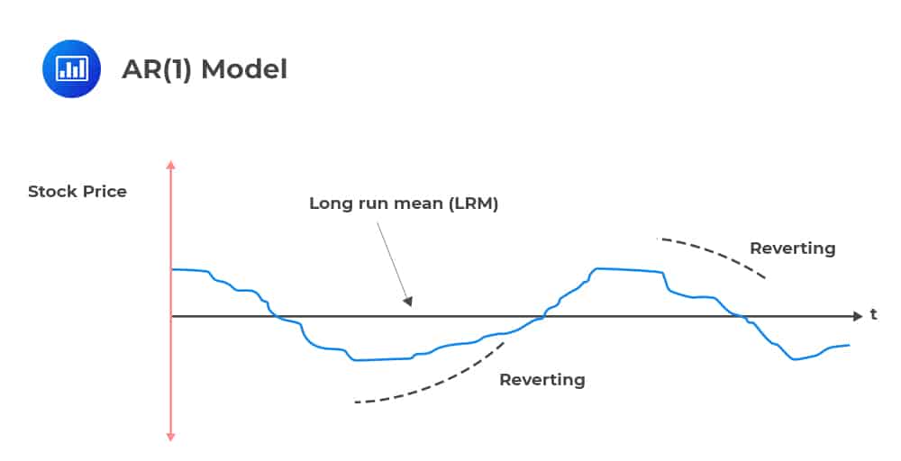 The simplest form of mean reversion can be illustrated by a first-order autoregressive process [AR(1)], where the current value is based on the immediately preceding value.
$$ \text{X}_{\text{t}+1}={\text{a}}+\text{b}{\text{X}}_{\text{t}}+{\text{e}}_{\text{t}+1} $$
The expected value of \(\text X_{\text t}\) as a function of period t information is:
$$ \text{E}\left[\text{X}_{\text{t}+1}\right]={\text{a}}+\text{b}{\text{X}}_{\text{t}} $$
We can restate this as:
$$ \text{E}\left[\text{X}_{\text{t}+1}\right]=\left(1-\text{b}\right)\times\cfrac{a}{1-{\text{b}}}+\text{b}{\text{X}}_{\text{t}} $$
The long-run mean of this model is evaluated as \(\left[\frac{a}{\left(1-{\text{b}}\right)}\right]\). The parameter of utmost interest in this long-run mean equation is b, often termed “the speed of reversion” parameter. There are two scenarios:
In GARCH (1,1), the long-run variance rate \(\left({\text{V}}_{\text{L}}\right)\) provides a “pull” mechanism towards the long-run average mean. Not that this is absent in the EWMA model due to a lack of the VL factor.
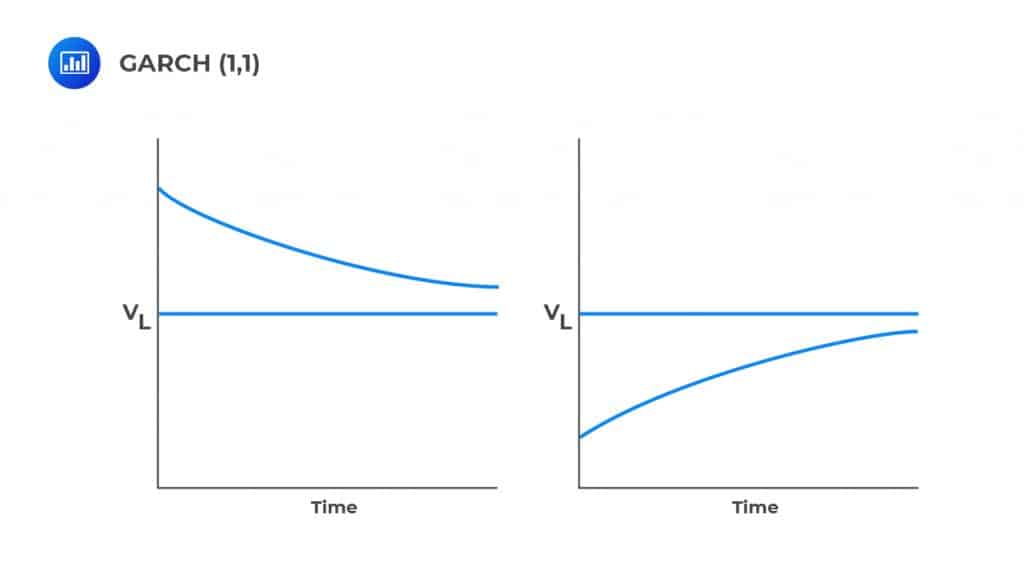 Consider the figure above. When the volatility is above the long-run average mean, \({\text{V}}_{\text{L}}\) “pulls” down toward it. On the other hand, when the volatility is below the long-run mean, \({\text{V}}_{\text{L}}\) pulls it towards the long-run mean. This tendency of the “pull” mechanism is termed as the mean reversion.
Therefore, GARCH (1,1) exhibits mean reversion, while EWMA does not. Mean reversion applies to market variables. More importantly, market variables that are traded should not exhibit predictable mean reversion to avoid arbitrage opportunities.
Notably, volatility cannot be traded, and thus it exhibits mean reversion. In this case, mean reversion implies that when the volatility is high, we do not expect to remain in that position forever but rather return to normal levels.
Our discussion has been based on approximating one-day volatility. We might want to know what will happen over a longer period, such as one year. To achieve this, we assume that the variance rate over T days is equivalent to T days times variance over one day. That is,
T-days variance rate=one-day variance rate×T
This means that volatility over days is equivalent to the volatility over one day multiplied by the square root of T days. That is
T-days volatility =one-day volatility×√T
Recall that this was true also for the VaR.
Assume that the daily variance rate is 0.000025. What is the 30-day volatility?
T−day =one-day volatility×√T=√0.000025×√30=0.0274=2.74%
Implied volatility is an alternative measure of volatility that is constructed using the option valuation. The options (both put and call) have payouts that are non-linear functions of the price of the underlying asset. For instance, the payout from the put option is given by:
$$ \text{max}\left(\text{K}-{\text{P}}_{\text{T}}\right) $$
Where:
\({\text{P}}_{\text{T}}\) is the price of the underlying asset,
\(\text{K}\) is the strike price, and
\(\text{T}\) is the maturity period.
Therefore, the price payout from an option is sensitive to the variance in the asset’s return.
The Black-Scholes-Merton model is commonly used for option pricing valuation. The model relates the price of an option to the risk-free rate of interest, the current price of the underlying asset, the strike price, time to maturity, and the variance of return. For instance, the price of the call option can be denoted by:
$$ \text{C}_{\text{t}}=\text{f}\left({\text{r}}_{\text{f}},{\text{T}},{\text{P}}_{\text{t}},{\sigma}^{2}\right) $$
Where:
\({\text{r}}_{\text{f}}\)= Risk-free rate of interest
\(\text{T}\)=Time to maturity
\({\text{P}}_{\text{t}}\)=Current price of the underlying asset
\({\sigma}^{2}\)=Variance of the return
The implied volatility σ relates the price of an option with the other three parameters. The implied volatility is an annualized value but can be converted by dividing by 252, which is an estimated number of trading days in a year. For instance, if annual volatility is 30%, then the daily implied volatility is 1.89% \(\left(=\cfrac{30\%}{\sqrt{252}}\right)\).
The difference between the implied volatility and historical volatility (such as the one estimated by GARCH(1,1) and EWMA models) is that implied volatility is forward-looking while historical volatility is backward-looking. For example, a one-month implied volatility indicates average volatilities over the next month.
Options are not actively traded, and thus finding reliable volatility is an uphill task. However, risk managers evaluate both implied and historical volatility.
The volatility index (VIX) measures the volatility of the S&P 500 over the coming 30 calendar days. VIX is constructed from a variety of options with different strike prices. VIX applies to a large variety of assets such as gold, but it is only applicable to highly liquid derivative markets and thus not applicable to most financial assets.
There are two main advantages of implied volatility over historical volatility:
On the other hand, implied volatility has its shortcomings:
Recall that in a delta-normal model, correlations between the daily asset returns are needed to compute the VaR or expected shortfall for a linear portfolio. Therefore, it is crucial to monitor correlations.
Updating the correlations is analogous to that of volatilities. Recall that while updating the volatilities, we use the variances. In the case of relationships, we use covariances. Now, assuming that mean of daily returns is zero, then the covariance is defined as the expectation of the product of returns.
According to the EWMA model, updating the correlation between returns X and Y is given by:
$$ \text{cov}_{\text{n}}={\lambda}{\text{cov}}_{\text{n}-1}+\left(1-{\lambda}\right){\text{x}}_{\text{n}-1}{\text{y}}_{\text{n}-1} $$
Where:
\(\text{cov}_{\text{n}}\): covariance for day n
\({\text{x}}_{\text{n}-1}\) and \({\text{y}}_{\text{n}-1}\): values of X and Y at day n.
Recall that for variables X and Y,
$$ \text{Corr}\left({\text{X}},{\text{Y}}\right)=\cfrac{\text{Cov}\left(\text{X},\text{Y}\right)}{{\sigma}_{\text{X}} {\sigma}_{\text{Y}}} $$
Where:
\(\text{Corr}\left({\text{X}},{\text{Y}}\right)\): correlation between variables X and Y;
\(\text{Cov}\left({\text{X}},{\text{Y}}\right)\): covariance between variables X and Y;
\({\sigma}_{\text{X}}\): standard deviation of X; and
\({\sigma}_{\text{Y}}\): standard deviation of Y.
Therefore, if the EWMA model has been used to estimate the standard deviations of the returns, we can comfortably estimate the correlation coefficient. However, the same value of \(\lambda\) is used while updating both variances and covariances for consistency.
Assume that recent volatilities for returns on X and Y are 2% and 5%, respectively. Their corresponding correlation coefficient is 0.4. Moreover, their recent returns are 3% and 4%, respectively.
Assuming \(\lambda\)=0.92, calculate the value of:
Solution
i. Updated volatilities
Denote the “recent” period by n-1. Now using the formula:
$$ { \sigma }_{ \text{n} }^{ 2 }=\left(1-{\lambda}\right){ \text{r} }^{2}_{ \text{n}-{1} }+{\lambda}{ \sigma }_{ \text{n}-1}^{ 2 } $$
The updated volatility for return X is given by:
$$ {\sigma}_{{\text{X}}_{\text{n}}}=\sqrt{(1-0.92)\times{0.03}^{2}+0.92\times{0.02}^{2}}=0.02098=2.098\% $$
And for return Y we have:
$$ {\sigma}_{{\text{Y}}_{\text{n}}}=\sqrt{(1-0.92)\times{0.04}^{2}+0.92\times{0.05}^{2}}=0.04927=4.927\% $$
ii. Updated correlation coefficient
Using the formula:
$$ \text{Corr}\left({\text{X}},{\text{Y}}\right)=\cfrac{\text{Cov}\left(\text{X},\text{Y}\right)}{{\sigma}_{\text{X}} {\sigma}_{\text{Y}}} $$
It intuitively means that:
$$ \begin{align*} \text{cov}_{\text{n}-1}&=\sigma _{ { \text{X} }_{ \text{n}-1 } }\times\sigma _{ { \text{Y} }_{ \text{n}-1 } }\times \text{Corr}\left({\text{X}_{\text{n}-1},\text{Y}_{\text{n}-1}}\right) \\ &=0.02\times0.05\times0.4\\ &=0.0004 \end{align*} $$
Now using:
$$ \text{cov}_{\text{n}}={\lambda}{\text{cov}}_{\text{n}-1}+\left(1-{\lambda}\right){\text{X}_{\text{n}-1}\text{Y}_{\text{n}-1}} $$
we have:
$$ \text{cov}_{\text{n}}={0.92}\times{0.0004}+\left(1-0.92\right)\times{0.03}\times{0.04}=0.000464 $$
And thus, the updated correlation coefficient is given by:
$$ \begin{align*} \text{corr}\left({\text{x}}_{\text{n}},{\text{y}}_{\text{n}}\right)&=\cfrac{\text{cov}_{\text{n}}}{\sigma _{ { \text{X} }_{ \text{n} } }\sigma _{ { \text{Y} }_{ \text{n} } }} \\ &=\cfrac{0.000464}{0.02098\times0.04927}=0.4489 \end{align*} $$
Practice Question
The current estimate of daily volatility is 2.3 percent. The closing price of an asset yesterday was CAD 46. Today, the asset ended the day at CAD 47.20. Using log-returns and the exponentially weighted moving average model with \({\lambda}\) = 0.94, determine the updated estimate of volatility.
- 2.319%
- 0.0537%
- 2.317%
- 2.315%
The correct answer is C.
The updated variance is given by:
$$ \text{h}_{\text{t}}={\lambda}\left(\text{current volatility}\right)^2+\left(1-{\lambda}\right)\left(\text{current return}\right)^{2} $$
Current volatility = 0.023
$$ \begin{align*} \text{Current log-return}&=\text{ln}47.2–\text{ln}46=3.85439–3.82864=0.02575 \\ \text{ht}&=0.94\left({0.023}^{2}\right)+\left(0.06\times{0.02575}^{2}\right)=0.000537 \\ \text{Updated estimate of volatility}&=\sqrt{0.000537}=0.02317 \end{align*} $$
Offered by AnalystPrep


