


Risk Data Aggregation and Reporting Pr ...
After completing this reading, you should be able to: Explain the potential benefits... Read More
After completing this reading, you should be able to:
A linear portfolio linearly depends on the changes in the values of its corresponding variables (risk factors). For instance, consider a portfolio consisting of 100 shares, each valued at USD 100. The change in portfolio value \(\left(\Delta{\text{P}}\right)\) is attributed to the change in stock (share price) which can be denoted by \(\Delta{\text{S}}\), and therefore the change in portfolio value is given by :
$$ \Delta{\text{P}}=100\Delta{\text{S}} $$
The value of the portfolio is USD 10,000 (=100×100). Now, if we introduce the effect of the interest rate, the change in the value of the portfolio will be given by:
$$ \Delta{\text{P}}=100\Delta{\text{r}} $$
Generally, consider a portfolio consisting of long and short positions in stocks. The change in a linear portfolio is given by:
$$ \Delta{\text{P}}=\sum _{ \text{i} }^{}{ { \text{n} }_{ \text{i} } } \Delta{\text{S}}_{\text{i}} $$
Where:
\({\text{n}}_{\text{i}}\) = Number of shares of stock i in the portfolio;
\({\text{S}}_{\text{i}}\) = The price of stock i.
Intuitively, the amount invested in stock i is \({\text{n}}_{\text{i}}\)\({\text{S}}_{\text{i}}\), and the price change is \(\Delta{\text{S}}_{\text{i}}\).
Now, if we multiply the above equation by \(\cfrac{{\text{S}}_{\text{i}}}{{\text{S}}_{\text{i}}} \) , we have:
$$ \Delta{\text{P}}=\sum _{ \text{i} }^{}{ { \text{n} }_{ \text{i} } } \Delta{\text{S}}_{\text{i}}\times\cfrac{{\text{S}}_{\text{i}}}{{\text{S}}_{\text{i}}}=\sum _{ \text{i} }^{}{ { \text{n} }_{ \text{i} } } \Delta{\text{S}}_{\text{i}}\cfrac{\Delta{\text{S}}_{\text{i}}}{{\text{S}}_{\text{i}}} $$
Let \({\text{q}}_{\text{i}}={\text{n}}_{\text{i}} {\text{S}}_{\text{i}} \) and \( \Delta{\text{r}}_{\text{i}}=\cfrac{\Delta{\text{S}}_{\text{i}}}{{\text{S}}_{\text{i}}} \) , then
$$ \Delta{\text{P}}=\sum _{ \text{i} }^{}{ { \text{q} }_{ \text{i} } } \Delta{\text{r}}_{\text{i}} $$
Note that \({\text{q}}_{\text{i}}\) is the amount invested in stock i, and \(\Delta{\text{r}}_{\text{i}}\)=\(\frac{\Delta{\text{S}}_{\text{i}}}{{\text{S}}_{\text{i}}} \) is the return on stock i.
Therefore, we can say the portfolio change is a linear function of change in stock price or change in stock returns.
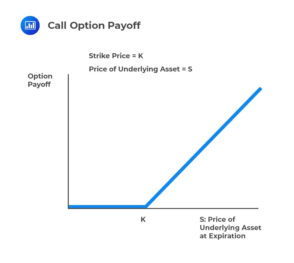
Nonlinear portfolios contain complex securities that are not linear. For instance, consider a portfolio made of call options. The payoff from the call option is nonlinear because the payoff is zero if the stock price is less than the strike price at maturity and S-K if the stock price is higher than the strike price K.
 Note, however, that a forward contract is an example of a derivative whose value is a linear function of the asset because even if the contracts do give a payoff, the holder is obligated to buy the asset at a future time T at agreed price K. As such, in case the asset provides no income, then the forward contract’s value is given by:
$$ {\text{S}}-{\text{PV}}\left(\text{K}\right) $$
Where S is the current asset price, and \({\text{PV}}\left(\text{K}\right)\) denote the present value of the future price K.
The figure below shows the relationship between the value of a forward contract and the underlying asset.
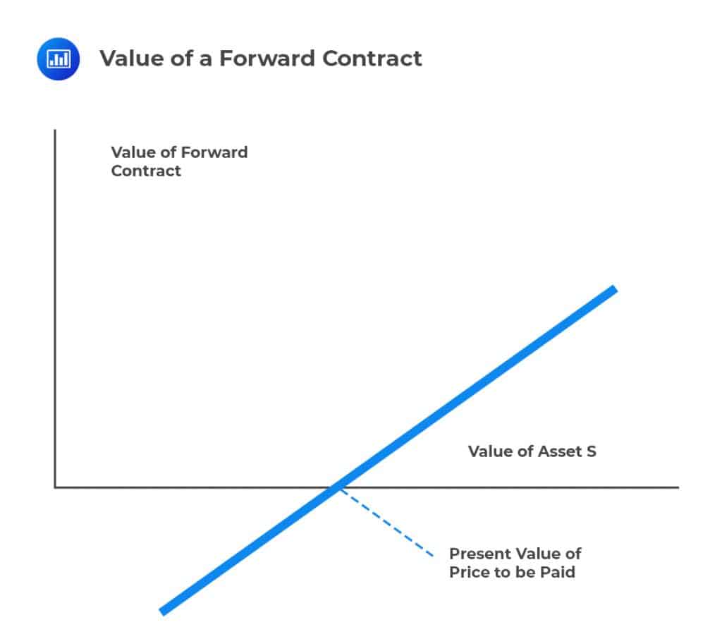
From the figure above, it is correct to say that a person who agrees to buy an asset at a future time is actually in a position to own the asset today but pay for it at a future time. Now, the value of owning the asset today is S, and the present value of what will be paid for the asset at the future time is PV(K). This proves the formula above for the value of the forward contract.
In general terms, the VaR of a linear derivative can be expressed as:
$$ \text{VaR}_{\text{linear derivative}}=\Delta\times{\text{VaR}}_{\text{Underlying factor}} $$
Where \({ \Delta }\) represents the sensitivity of the derivative’s price to the price of the underlying asset. It is usually expressed as a percentage.
Suppose the permitted lot size of S&P 500 futures contracts is 300 and multiples thereof, what is the VaR of an S&P 500 futures contract?
$$ \text{VaR}_{\text{S&P500futures c.}}=300\times{\text{VaR}}_{\text{S&P500 index}} $$
Historical simulation is used to calculate one-day VaR and ES. However, for longer periods T it is assumed that,
$$ \begin{align*} \text{VaR}\left({ \text{T} },{ \text{X} }\right)&=\sqrt{ \text{T} }\times \text{VaR}\left(1,{ \text{X} }\right) \\ \text{ES}\left({ \text{T} },{ \text{X} }\right)&=\sqrt{ \text{T} }\times \text{ES}\left(1,{ \text{X} }\right) \end{align*} $$
\(\text{VaR}\left({ \text{T} },{ \text{X} }\right)\) = Value at risk for a time horizon of T days and confidence level X.
\(\text{ES}\left({ \text{T} },{ \text{X} }\right)\) = Expected shortfall for a time horizon of T days and confidence level X.
The above estimates assume that the portfolios’ changes are normally distributed with a mean of zero and independent of each other.
The historical simulation procedure involves the following steps:
Risk factors are broadly classified into:
A portfolio is assumed to depend on many risk factors. For clarity, let us assume that three risk factors (exchange rates, interest rates, and stock price) over the past 300 days (longer periods such as 500 days are usually considered.) The most recent 301 days of historical data is as follows:
$$ \begin{array}{c|c|c|c|c} \textbf{Day} & {\textbf{Stock Price} \\ \textbf{(USD)} } & {\textbf{Exchange} \\ \textbf{rates} \\ \textbf{(USD/CAD)} } & {\textbf{Interest} \\ \textbf{rate (%)} } & {\textbf{Portfolio} \\ \textbf{Value} \\ \textbf{(USD} \\ \textbf{millions)}} \\ \hline {0} & {30} & {1.3901} & {3.51} & {60.0} \\ \hline {1} & {34} & {1.4000} & {2.64} & {62.5} \\ \hline {2} & {40} & {1.3921} & {2.52} & {61.25} \\ \hline {..} & {..} & {..} & {..} & {..} \\ \hline {298} & {42} & {1.3876} & {2.40} & {65.0} \\ \hline {299} & {40} & {1.3910} & {2.45} & {60.25} \\ \hline {300} & {60} & {1.4021} & {2.50} & \textbf{71.25} \end{array} $$
Assuming that today is the 300th day, we need to know what will happen between today and tomorrow (301st day). To achieve this, we use the above data to create 300 scenarios (that is why we have 301-day historical data).
In the first scenario, we will assume that the risk factors behave between the days 300 and 301 in a similar manner as they did between days 0 and 1. For instance, in the first scenario, the stock price increased by \(13\% \left(=\frac{34}{30}-1\right)\), and therefore the stock price on day 301 is USD 68 \( \left[=\left(\frac{34}{30}-1\right)\times60\right] \). For the exchange rate, it increased by 0.7% \(\left(=\frac{1.400}{1.3901}-1\right)\), and thus, we expect the exchange rate for the 301st day to be 1.4121 \( \left(=1.4021\left[\frac{1.400}{1.3901}-1\right]\right) \). For the interest rate, it decreased by 0.87% (2.64%-3.51%) and thus 301st interest rate is 1.63% (2.50%-0.87%).
The calculation of the values of the second and subsequent scenarios’ risk factors is similar to the first scenario calculation. For the second scenario, assume that the risk factors behave in a similar manner as they did between days 1 and 2. This will create the following table.
$$ \begin{array}{c|c|c|c|c|c} \textbf{Scenario} & {\textbf{Stock Price} \\ \textbf{(USD)} } & {\textbf{Exchange} \\ \textbf{rates} \\ \textbf{(USD/CAD)} } & {\textbf{Interest} \\ \textbf{rate (%)} } & {\textbf{Portfolio} \\ \textbf{Value} \\ \textbf{(USD} \\ \textbf{millions)}} & \textbf{Loss} \\ \hline {1} & {68} & {1.4121} & {3.37} & {70.25} & {1.0} \\ \hline {2} & {71} & {1.3922} & {2.38} & {72.15} & {0.9} \\ \hline {..} & {..} & {..} & {..} & {..} \\ \hline {299} & {57.14} & {1.3910} & {2.55} & {71.25} & {0} \\ \hline {300} & {90} & {1.4021} & {2.55} & {73.25} & {2.0} \end{array} $$
The risk factor values for the scenario table are directly calculated from the historical data table. The scenario portfolio values are generated based on the risk factors. We assume that the current portfolio value is USD 71.25 million (300th day’s value). After generating the portfolio values, we calculate the losses while attaching a negative to create a loss distribution.
Assume that the first scenario’s portfolio value is 70.25, 72.15 for the second scenario, and so on. Therefore, the loss for the first portfolio is 1.00 (=71.25-70.25), and the second scenario is 0.9 (71.25-72.15), and so on.
In order to calculate the VaR and the expected shortfall, we ought to arrange the scenario losses from the largest to the smallest. Assume that in our example, we wish to calculate one day VaR and ES at a 99% confidence interval. The sorted losses are as follows:
$$ \begin{array}{c|c} \textbf{Scenario} & \textbf{Loss} \\ \hline {200} & {3.9} \\ \hline {10} & {3.0} \\ \hline {25} & {2.5} \\ \hline {100} & {2.0} \\ \hline {…} & {…} \\ \hline {…} & {…} \end{array} $$
In this case, VaR is equivalent to third-worst loss since the third-worst loss is the first percentile point of the distribution, i.e., \(\cfrac{3}{100}=0.01\). Therefore, VaR=2.5 million.
By definition, the expected shortfall is calculated as the average of the losses that are worse than the VaR. In this case,
$$ \text{ES}=\cfrac{1}{2}\left(3.9+3.0\right)=3.45 \text{ million } $$
The following are hypothetical ten worst returns for an asset B from 120 days of data for 6 months. Find the 1-day 5% VaR and the ES for B.
-3.45%, -14.12%, -15.72%, -10.92%, -5.50%, -3.56%, -6.90%, -2.50%, -5.30%, -4.31%.
First, we rearrange starting with the worst day, to the least bad day, as shown below:
-15.72%, -14.12%, -10.92%, -6.90%, -5.50%, -5.30%, -4.31%, -3.56%, -3.45%, -2.50%.
The VaR corresponds to the \((5\%\times120)\)=6th worst day = -5.30%. However, recall that VaR need not be represented as a negative.
This implies that there is a 95% probability of getting at most 5.3% loss.
The expected shortfall (ES) is calculated as the average of the losses that are worse than the VaR. In this case,
$$ \text{ES}=\cfrac{\left(15.72\%+14.12\%+10.92\%+6.90\%+5.50\%\right)}{5}=10.63\% $$
Before we look at the delta-normal model, we will biefly look at the full revaluation approach. Under this approach the VaR of a portfolio is established by fully repricing the portfolio under a set of scenarios over a period of time.
However, a full revaluation of a portfolio for many scenarios is a time-consuming activity. One approach to address this challenge is to use Greek letters. The Greek letters are the hedging parameters used by analysts to quantify and manage risks.
One of the crucial Greek letter deltas \(({\delta})\) is defined as:
$$ {\delta}=\cfrac{\Delta{\text{P}}}{\Delta{\text{S}}} $$
Where \(\Delta{\text{S}}\) is a small change in risk factors such as stock price and \(\Delta {\text P}\) the corresponding change in the portfolio value. Therefore, delta can be defined as a change of the portfolio value with respect to the change in the risk factor.
For instance, consider stock price as a risk factor. If the delta of a portfolio with respect to the stock price is USD 100, it implies that the portfolio value changes by USD 100 if the stock price changes by 1 USD.
From the delta formula, we express the change in the portfolio value as :
$$ \Delta{\text{P}}=\delta{\Delta{\text{S}}} $$
Generally, if we have multiple risk factors, we find each risk factor’s effect and sum it up. That is, if we have i risk factors, then change in the portfolio would be:
$$ \Delta{\text{P}}=\sum _{ \text{i} }^{}{ { \delta }_{ \text{i} } } \Delta{\text{S}}_{\text{i}} $$
However, the delta concept gives relatively accurate estimates in linear portfolios as compared to nonlinear portfolios.
The accuracy of nonlinear portfolios can be enhanced by including another Greek letter gamma \((\gamma)\) so that the delta-gamma formula is given by:
$$ \Delta{\text{P}}=\delta{\Delta{\text{S}}}+\cfrac{1}{2} {\gamma} \left(\Delta{\text{S}}\right)^{2} $$
In case of multiple risk factors, the above equation changes to:
$$ \Delta{\text{P}}=\sum _{ \text{i} }^{}{ { \delta }_{ \text{i} } } \Delta{\text{S}}_{\text{i}}+\cfrac{1}{2}\sum _{ \text{i} }^{}{ { \gamma }_{ \text{i} } }\left(\Delta{\text{S}}_{\text{i}}\right)^{2}$$
The delta-normal model is based on the equation (as seen earlier):
$$ \Delta{\text{P}}=\sum _{ \text{i} }^{}{ { \delta }_{ \text{i} } } \Delta{\text{S}}_{\text{i}} $$
Note that this equation gives an exact value in a linear portfolio and an approximate value in nonlinear portfolios.
 Also, recall that we have two types of risk factors:
To accommodate both types of risk factors, the equation above is written as:
$$ \Delta{\text{P}}=\sum _{ \text{i} }^{}{ { \text{a} }_{ \text{i} } } {\text{x}}_{\text{i}} $$
For risk factors where percentage changes are used, \({ \text{a} }_{ \text{i} }=\frac{\Delta{ \text{S} }_{ \text{i} }}{{ \text{S} }_{ \text{i} }} \) and \({ \text{x} }_{ \text{i} }={ \delta }_{ \text{i} } { \text{S} }_{ \text{i} }\).
And for the risk factors where actual changes are considered \({ \text{a} }_{ \text{i} }=\Delta{ \text{S} }_{ \text{i} }\) and \({ \text{x} }_{ \text{i} }={ \delta }_{ \text{i} } \).
From the resulting equations, the mean and the standard deviation of the change in portfolio value can be calculated as:
$$ \begin{align*} { \mu }_{\text{P}}&=\sum _{ \text{i}=1 }^{\text{n}}{ { \text{a} }_{ \text{i} } }{ \mu }_{\text{i}} \\ \sigma _{ \text{P} }^{2}&=\sum _{ \text{i}=1 }^{ n }{ \sum _{ \text{j}=1 }^{ \text{n} }{ \text{a}_{ \text{i} }\text{a}_{ \text{j} }{ { \rho }_{ \text{ij} }\sigma }_{ \text{i} }{ \sigma }_{ \text{j} } } } \end{align*} $$
Where:
\({ \mu }_{\text{i}}\) and \({ \sigma }_{\text{i}}\) are the mean and standard deviation of \({ \text{x} }_{ \text{i} }\), respectively.
\({ \rho }_{ \text{ij} }\) is the coefficient of correlation between \({ \text{x} }_{ \text{i} }\) and \({ \text{x} }_{ \text{j} }\).
The formula for the standard deviation can be written as:
$$ \sigma _{ \text{P} }^{2}=\text{a} _{ \text{i} }^{2}\sigma_{ \text{i} }^{2}+2\sum _{ \text{i>j} }^{ }\text{a}_{ \text{i} }\text{a}_{ \text{j} }{ { \rho }_{ \text{ij} }\sigma }_{ \text{i} }{ \sigma }_{ \text{j} } $$
Assuming that the portfolio changes are normally distributed, we can comfortably compute VaR and ES. Remember that the VaR is given by:
$$\begin{align*} \text{VaR}&={\mu}_{\text{P}}+{\sigma}_{\text{P}} {\text{U}} \\ {ES}&={\mu}_{\text{P}}+{\sigma}_{\text{P}}\left(\cfrac { { \text{e} }^{ -\frac { { \text{U} }^{ 2 } }{ 2 } } }{ \left( 1-{ \text{X} } \right) \sqrt { 2\pi } } \right) \end {align*}$$
Where:
X = Confidence level
U = Point on the normal distribution where X is exceeded
For instance, if X=95% then U=\({ \Phi }^{-1} (0.05)=-1.645.\)
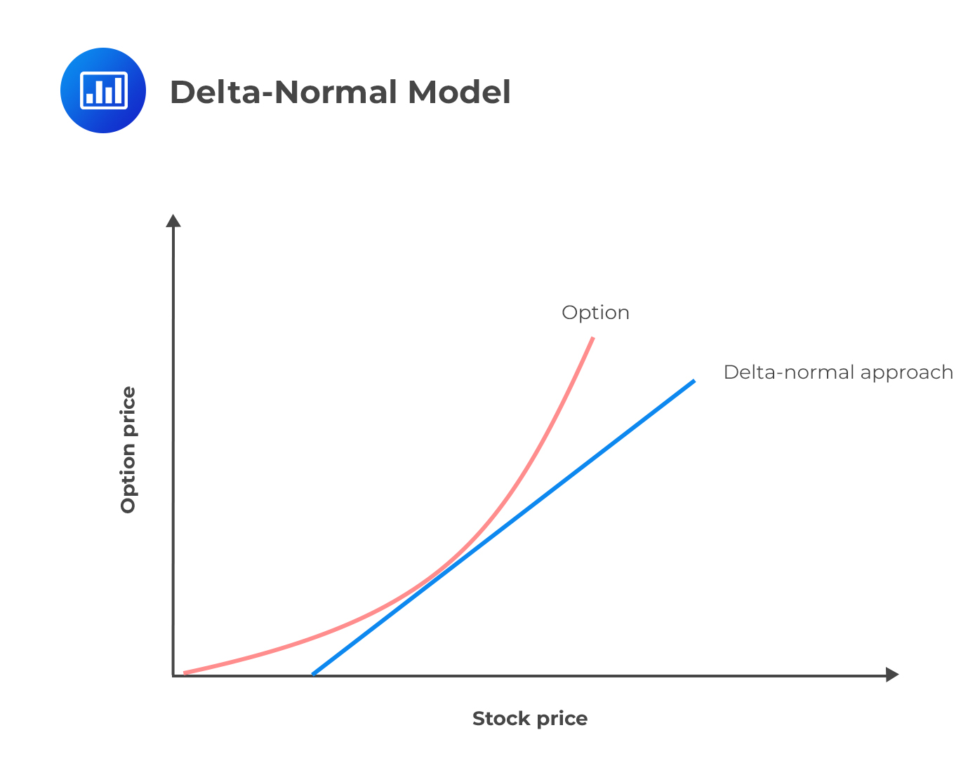
At this point, you might guess where the name “delta-normal” comes from: the model uses deltas of the risk factors and assumes that the portfolio changes are normally distributed.
A typical assumption is that the mean change in the risk factor is zero. This assumption is sometimes not reasonable but is useful when dealing with short time periods. This is because the mean is less than the standard deviation for short periods when dealing with portfolio value changes. As such, VaR and ES are given by:
$$ \begin{align*} \text{VaR}& ={\sigma}_{\text{P}} {\text{U}} \\ \text{ES}& ={\sigma}_{\text{P}}\left(\cfrac { { \text{e} }^{ -\frac { { \text{U} }^{ 2 } }{ 2 } } }{ \left( 1-{ \text{X} } \right) \sqrt { 2\pi } } \right) \end{align*} $$
The investment return over a period of time has a normal loss distribution with a mean of -100 and a variance of 400.
Using the delta-normal model, calculate the 99% Expected Shortfall and the 99% VaR of the loss distribution.
$$\begin{align*}\mathrm{ES}&=\sigma_{\mathrm{p}}\left(\frac{\mathrm{e}^{-\frac{\mathrm{U}^{2}}{2}}}{(1-\mathrm{x}) \sqrt{2 \pi}}\right)\\ &=20\left(\frac{\mathrm{e}^{-\frac{2.33^{2}}{2}}}{(1-0.99) \sqrt{2 \pi}}\right)=52.85 \end{align*}$$
Where X is the confidence level and U is the point on the normal distribution where X is exceeded
The 99% VaR is given by:
$$\text{VaR}=\sigma_{\mathrm{p}} \text{U} =20 \times(-2.33)=-46.6$$
The method has several disadvantages, chief among them being that:
 For large changes in a nonlinear derivative, we must use the delta + gamma approximation, or full revaluation as we had discussed earlier.
Monte Carlo approach is similar to that of the historical simulation. It is noteworthy, though, that the Monte Carlo simulation produces scenarios by randomly selecting samples from the distribution assumed for the risk factors instead of using historical data. Monte Carlo simulations work for both linear and nonlinear portfolios.
Now, if for instance, we assume that risk factor changes have a multivariate normal distribution (as in delta-normal), Monte Carlo procedure is as follows:
Step 1: Calculate the value of the portfolio today using the current values of the risk factors.
Step 2: Sample once from the multivariate normal probability distribution of \(\Delta{\text{x}}_{\text{i}}\). Sampling should be consistent with the assumed standard deviations and correlations, which are usually approximated from historical data.
Step 3: Using the sample values of \(\Delta{\text{x}}_{\text{i}}\), determine the values of the risk factors at the end of the period being considered (such as one day).
Step 4: Revalue the portfolio using these new risk factor values.
Step 5: Subtract the revaluated portfolio from the current portfolio value to determine the loss.
Step 6: Repeat step 2 to step 5 multiple times to come up with a probability distribution for the loss.
For instance, if a total of 500 trials are conducted in a Monte Carlo simulation, then 99% VaR for the period under consideration will be the fifth-worst loss. Therefore, the expected shortfall will be the average of the four losses worse than VaR.
Like other approaches, Monte Carlo simulation computes one-day VaR, and therefore, the following equations apply when we want to compute T-day time horizon VaR and ES:
$$ \begin{align*} \text{VaR}\left({ \text{T} },{ \text{X} }\right)&=\sqrt{ \text{T} }\times \text{VaR}\left(1,{ \text{X} }\right) \\ \text{ES}\left({ \text{T} },{ \text{X} }\right)&=\sqrt{ \text{T} }\times \text{ES}\left(1,{ \text{X} }\right) \end{align*} $$
Monte Carlo simulation is slow because it is computationally intensive. This can be explained by the fact that portfolios considered are usually huge, and evaluating each one of them in each trial is quite time-consuming. To address this challenge, the delta-gamma approach can be used (as discussed earlier) to determine the change in the portfolio value. This is called partial simulation.
Delta-normal model assumes normal distribution for the risk factors. However, Monte Carlo simulation uses any distribution for the risk factors only if the correlation between the risk factors can be defined.
To execute the Monte Carlo simulation or delta-normal model, an approximation of the standard deviations and correlations of either percentage or actual changes of the risk factors is necessary. The approximation of these parameters is made using recent historical data. More weights can be applied to more recent data using models such as GARCH (1,1), which we will see in the following chapter.
In the case of stressed VaR and ES, standard deviations and correlations should be estimated from the past period, which would be considered stressful to the current portfolio.
During the stressed market conditions, standard deviations as well as correlations increase. This phenomenon was witnessed during the 2007-2008 financial crisis, where default rates of mortgages increased all over the US.
Therefore, correlations in a high volatility period are quite different from those of normal market conditions. This phenomenon is referred to as a correlation breakdown. As such, when calculating VaR or ES, risk managers might need to determine what will happen in extreme market conditions.
Worst-case scenario analysis focuses on extreme losses at the tail end of a distribution. First, firms assume that an unfavorable event is certain to occur. They then attempt to establish its possible worst outcomes.
WCS analysis dissects the tail further to establish the range of worst-case losses that could be incurred. For example, within the lowest 5% of returns, we can construct a “secondary” distribution that specifies the 1% WCS return.
WCS analysis complements the VaR, and here is how. Recall that the VaR specifies the minimum loss for a given percentage, but it stops short of establishing the severity of losses in the tail. WCS analysis goes a step further to describe the distribution of extreme losses more precisely.
Practice Questions
Question 1
A risk manager wishes to calculate the VaR for a Nikkei futures contract using the historical simulation approach. The current price of the contract is 955, and the multiplier is 250. For the last 300 days, the following return data has been recorded:
-7.8%, -7.0%, -6.2%, -5.2%, -4.6%, -3.2%, -2.0%, …, 3.8%, 4.2%, 4.8%, 5.1%, 6.3%, 6.8%, 7.0%
What is the VaR of the position at 99% using the historical simulation methodology?
A. $12,415
B. $16,713
C. $18,623
D. $14,803
The correct answer is D.
The 99% return among 300 observations would be the third-worst observation among the returns \(((1-0.99)*300=3)\).
Among the returns given above, the third-worst return is −6.2%. As such,
$$ \text{VaR}_{(99\%)} = 6.2\% \times 955 \times 250 = 14,802.50 $$
A is incorrect. This answer incorrectly uses the fourth-worst observation as the 99% return among 300 observations.
B is incorrect. This answer incorrectly uses the second-worst observation as the 99% return among 300 observations.
C is incorrect. This answer incorrectly uses the worst observation as the 99% return among 300 observations.
Question 2
Bank X and Bank Y are two competing investment banks that are calculating the 1-day 99% VaR for an at-the-money call on a non-dividend-paying stock with the following information:
- Current stock price: USD 100
- Estimated annual stock return volatility: 20%
- Current Black-Scholes-Merton option value: USD 4.80
- Option delta: 0.7
To compute VaR, Bank X uses the linear approximation method, while Bank Y uses a Monte Carlo simulation method for full revaluation. Which bank will estimate a higher value for the 1-day 99% VaR?
- Bank X.
- Bank Y.
- Both will have the same VaR estimate.
- Insufficient information to determine.
The correct answer is A.
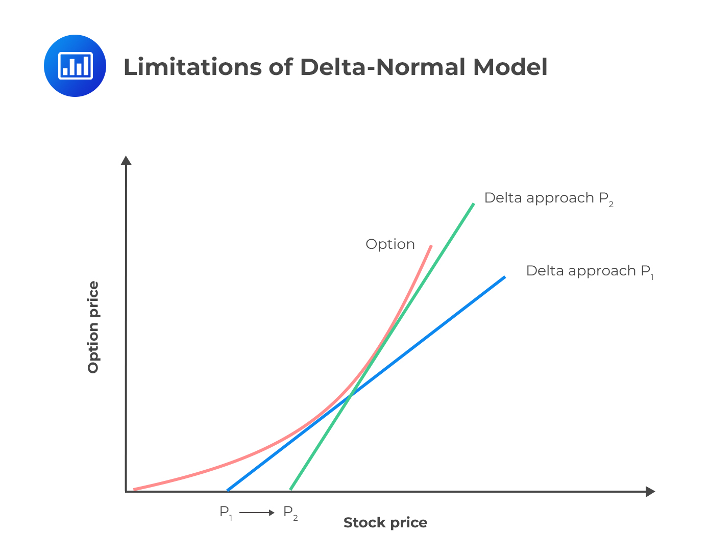
The option’s return function is convex with respect to the value of the underlying. Therefore the linear approximation method will always underestimate the true value of the option for any potential change in price. As such, the VaR will always be higher under the linear approximation method than a full revaluation conducted by Monte Carlo simulation analysis. The difference is the bias resulting from the linear approximation, and this bias increases in size with the change in the option price and with the holding period.
As a quick summary, linear approximation underestimates true price of the option (see the graph below), and as such, overestimates the value-at-risk.
Offered by AnalystPrep


