


Using Futures for Hedging
After completing this reading, you should be able to: Define and differentiate between... Read More

After completing this reading, you should be able to:
Hypothesis testing is defined as a process of determining whether a hypothesis is in line with the sample data. Hypothesis testing tries to test whether the observed data of the hypothesis is true. Hypothesis testing starts by stating the null hypothesis and the alternative hypothesis. The null hypothesis is an assumption of the population parameter. On the other hand, the alternative hypothesis states the parameter values (critical values) at which the null hypothesis is rejected. The critical values are determined by the distribution of the test statistic (when the null hypothesis is true) and the size of the test (which gives the size at which we reject the null hypothesis).
The elements of the test hypothesis include:
As stated earlier, the first stage of the hypothesis test is the statement of the null hypothesis. The null hypothesis is the statement concerning the population parameter values. It brings out the notion that “there is nothing about the data.”
The null hypothesis, denoted as H0, represents the current state of knowledge about the population parameter that’s the subject of the test. In other words, it represents the “status quo.” For example, the U.S Food and Drug Administration may walk into a cooking oil manufacturing plant intending to confirm that each 1 kg oil package has, say, 0.15% cholesterol and not more. The inspectors will formulate a hypothesis like:
H0: Each 1 kg package has 0.15% cholesterol.
A test would then be carried out to confirm or reject the null hypothesis.
Other typical statements of H0 include:
$$H_0:\mu={\mu}_0$$
$$H_0:\mu≤{\mu}_0$$
Where:
\(μ\) = true population mean and,
\(μ_0\)= the hypothesized population mean.
The alternative hypothesis, denoted H1, is a contradiction of the null hypothesis. The null hypothesis determines the values of the population parameter at which the null hypothesis is rejected. Thus, rejecting the H0 makes H1 valid. We accept the alternative hypothesis when the “status quo” is discredited and found to be untrue.
Using our FDA example above, the alternative hypothesis would be:
H1: Each 1 kg package does not have 0.15% cholesterol.
The typical statements of H1 include:
$$H_1:\mu \neq {\mu}_0$$
$$H_1:\mu > {\mu}_0$$
Where:
\(μ\) = true population mean and,
\(μ_0\)= the hypothesized population mean.
Note that we have stated the alternative hypothesis, which contradicted the above statement of the null hypothesis.
A test statistic is a standardized value computed from sample information when testing hypotheses. It compares the given data with what we would expect under the null hypothesis. Thus, it is a major determinant when deciding whether to reject H0, the null hypothesis.
We use the test statistic to gauge the degree of agreement between sample data and the null hypothesis. Analysts use the following formula when calculating the test statistic.
$$ \text{Test Statistic}= \frac{(\text{Sample Statistic–Hypothesized Value})}{(\text{Standard Error of the Sample Statistic})}$$
The test statistic is a random variable that changes from one sample to another. Test statistics assume a variety of distributions. We shall focus on normally distributed test statistics because it is used hypotheses concerning the means, regression coefficients, and other econometric models.
We shall consider the hypothesis test on the mean. Consider a null hypothesis \(H_0:μ=μ_0\). Assume that the data used is iid, and asymptotic normally distributed as:
$$\sqrt{n} (\hat{\mu}-\mu) \sim N(0, {\sigma}^2)$$
Where \({\sigma}^2\) is the variance of the sequence of the iid random variable used. The asymptotic distribution leads to the test statistic:
$$T=\frac{\hat{\mu}-{\mu}_0}{\sqrt{\frac{\hat{\sigma}^2}{n}}}\sim N(0,1)$$
Note this is consistent with our initial definition of the test statistic.
The following table gives a brief outline of the various test statistics used regularly, based on the distribution that the data is assumed to follow:
$$\begin{array}{ll}
\textbf{Hypothesis Test} & \textbf{Test Statistic}\\
\text{Z-test} & \text{z-statistic} \\
\text{Chi-Square Test} & \text{Chi-Square statistic}\\
\text{t-test} & \text{t-statistic} \\
\text{ANOVA} & \text{F-statistic}\\
\end{array}$$
We can subdivide the set of values that can be taken by the test statistic into two regions: One is called the non-rejection region, which is consistent with H0 and the rejection region (critical region), which is inconsistent with H0. If the test statistic has a value found within the critical region, we reject H0.
Just like with any other statistic, the distribution of the test statistic must be specified entirely under H0 when H0 is true.
While using sample statistics to draw conclusions about the parameters of the population as a whole, there is always the possibility that the sample collected does not accurately represent the population. Consequently, statistical tests carried out using such sample data may yield incorrect results that may lead to erroneous rejection (or lack thereof) of the null hypothesis. We have two types of errors:
Type I error occurs when we reject a true null hypothesis. For example, a type I error would manifest in the form of rejecting H0 = 0 when it is actually zero.
Type II error occurs when we fail to reject a false null hypothesis. In such a scenario, the test provides insufficient evidence to reject the null hypothesis when it’s false.
The level of significance denoted by α represents the probability of making a type I error, i.e., rejecting the null hypothesis when, in fact, it’s true. α is the direct opposite of β, which is taken to be the probability of making a type II error within the bounds of statistical testing. The ideal but practically impossible statistical test would be one that simultaneously minimizes α and β. We use α to determine critical values that subdivide the distribution into the rejection and the non-rejection regions.
The decision to reject or not to reject the null hypothesis is based on the distribution assumed by the test statistic. This means if the variable involved follows a normal distribution, we use the level of significance (α) of the test to come up with critical values that lie along with the standard normal distribution.
The decision rule is a result of combining the critical value (denoted by \(C_α\)), the alternative hypothesis, and the test statistic (T). The decision rule is to whether to reject the null hypothesis in favor of the alternative hypothesis or fail to reject the null hypothesis.
For the t-test, the decision rule is dependent on the alternative hypothesis. When testing the two-side alternative, the decision is to reject the null hypothesis if \(|T|>C_α\). That is, reject the null hypothesis if the absolute value of the test statistic is greater than the critical value. When testing on the one-sided, decision rule, reject the null hypothesis if \(T<C_α\) when using a one-sided lower alternative and if \(T>C_α\) when using a one-sided upper alternative. When a null hypothesis is rejected at an α significance level, we say that the result is significant at α significance level.
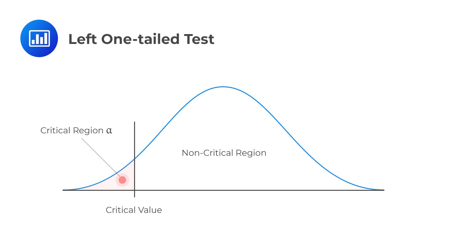
Note that prior to decision-making, one must decide whether the test should be one-tailed or two-tailed. The following is a brief summary of the decision rules under different scenarios:
H1: parameter < X
Decision rule: Reject H0 if the test statistic is less than the critical value. Otherwise, do not reject H0.
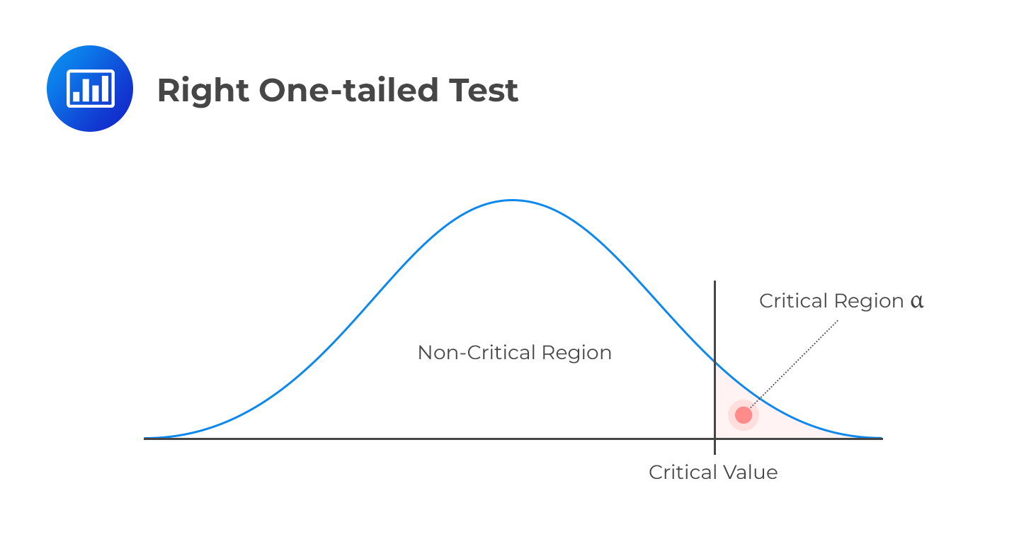
 Right One-tailed Test
H1: parameter > X
Decision rule: Reject H0 if the test statistic is greater than the critical value. Otherwise, do not reject H0.
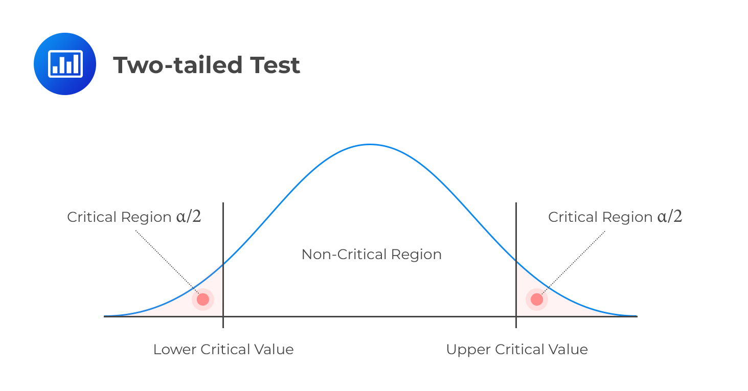
 Two-tailed Test
H1: parameter ≠ X (not equal to X)
Decision rule: Reject H0 if the test statistic is greater than the upper critical value or less than the lower critical value.
 Consider, α=5%. Consider a one-sided test. The rejection regions are shown below:
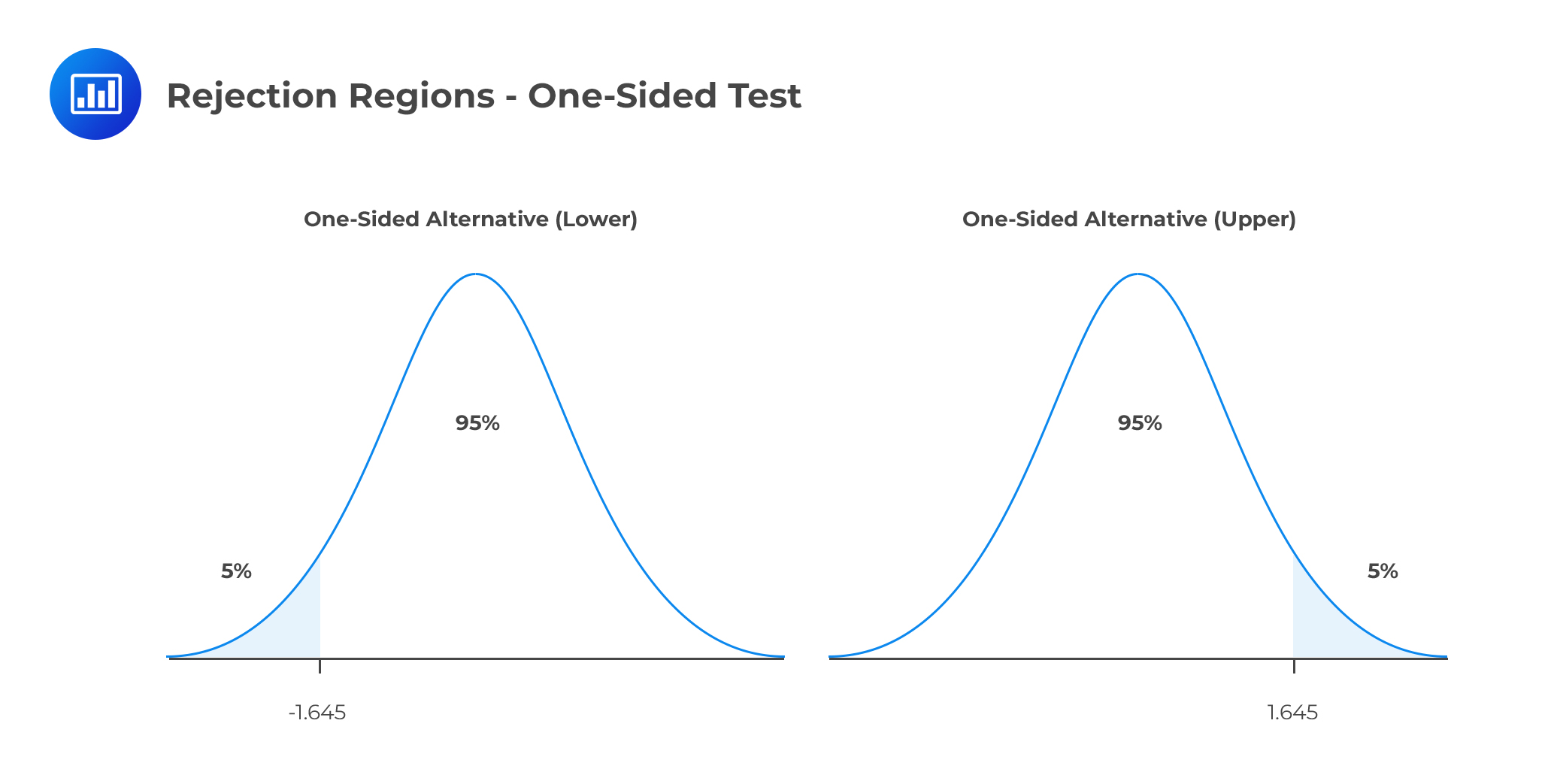 The first graph represents the rejection region when the alternative is one-sided lower. For instance, the hypothesis is stated as:
H0: μ < μ0 vs. H1: μ > μ0.
The second graph represents the rejection region when the alternative is a one-sided upper. The null hypothesis, in this case, is stated as:
H0: μ > μ0 vs. H1: μ < μ0.
Consider the returns from a portfolio \(X=(x_1,x_2,\dots, x_n)\) from 1980 through 2020. The approximated mean of the returns is 7.50%, with a standard deviation of 17%. We wish to determine whether the expected value of the return is different from 0 at a 5% significance level.
Solution
We start by stating the two-sided hypothesis test:
H0: μ =0 vs. H1: μ ≠ 0
The test statistic is:
$$T=\frac{\hat{\mu}-{\mu}_0}{\sqrt{\frac{\hat{\sigma}^2}{n}}} \sim N(0,1)$$
In this case, we have,
\(n\)=40
\(\hat{μ}\)=0.075
\(μ_0\)=0
\(\hat{\sigma}^2\)=0.172
So,
$$T=\frac{0.075-0}{\sqrt{\frac{0.17^2}{40}}} \approx 2.79$$
At the significance level, \(α=5\%\),the critical value is \(±1.96\). Since this is a two-sided test, the rejection regions are ( \(-\infty,-1.96\) ) and (\(1.96, \infty \) ) as shown in the diagram below:
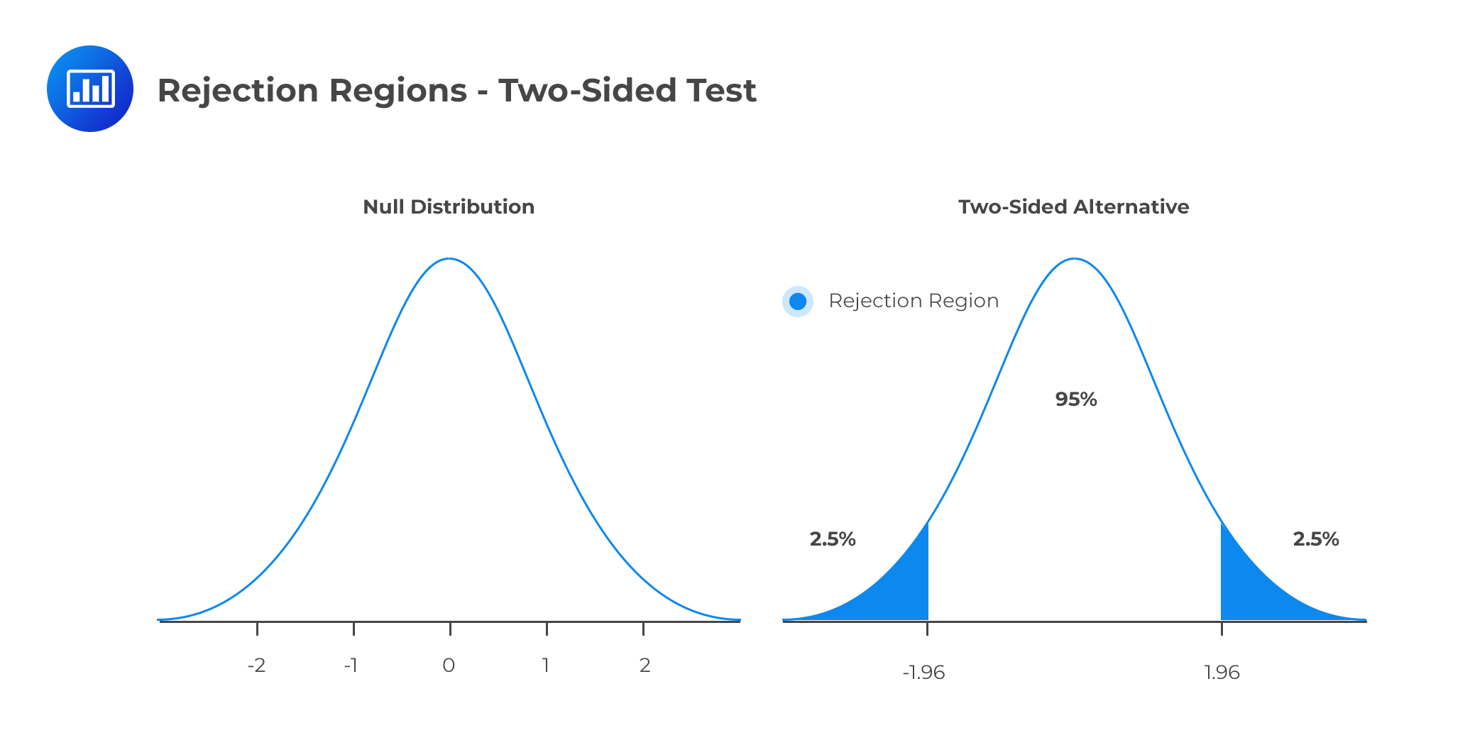 Since the test statistic (2.79) is higher than the critical value, then we reject the null hypothesis in favor of the alternative hypothesis.
The example above is an example of a Z-test (which is mostly emphasized in this chapter and immediately follows from the central limit theorem (CLT)). However, we can use the Student’s t-distribution if the random variables are iid and normally distributed and that the sample size is small (n<30).
In Student’s t-distribution, we used the unbiased estimator of variance. That is:
$$s^2=\frac{\hat{\mu}-{\mu}_0}{\sqrt{\frac{s^2}{n}}}$$
Therefore the test statistic for \(H_0=μ_0\) is given by:
$$T=\frac{\hat{\mu}-{\mu}_0}{\sqrt{\frac{s^2}{n}}} \sim t_{n-1}$$
The power of a test is the direct opposite of the level of significance. While the level of relevance gives us the probability of rejecting the null hypothesis when it’s, in fact, true, the power of a test gives the probability of correctly discrediting and rejecting the null hypothesis when it is false. In other words, it gives the likelihood of rejecting H0 when, indeed, it’s false. Denoting the probability of type II error by \(\beta\), the power test is given by:
$$ \text{Power of a Test}=1–\beta $$
The power test measures the likelihood that the false null hypothesis is rejected. It is influenced by the sample size, the length between the hypothesized parameter and the true value, and the size of the test.
A confidence interval can be defined as the range of parameters at which the true parameter can be found at a confidence level. For instance, a 95% confidence interval constitutes the set of parameter values where the null hypothesis cannot be rejected when using a 5% test size. Therefore, a 1-α confidence interval contains values that cannot be disregarded at a test size of α.
It is important to note that the confidence interval depends on the alternative hypothesis statement in the test. Let us start with the two-sided test alternatives.
$$ H_0:μ=0$$
$$H_1:μ≠0$$
Then the \(1-α\) confidence interval is given by:
$$\left[\hat{\mu} -C_{\alpha} \times \frac{\hat {\sigma}}{\sqrt{n}} ,\hat{\mu} + C_{\alpha} \times \frac{\hat {\sigma}}{\sqrt{n}} \right]$$
\(C_α\) is the critical value at \(α\) test size.
Consider the returns from a portfolio \(X=(x_1,x_2,…, x_n)\) from 1980 through 2020. The approximated mean of the returns is 7.50%, with a standard deviation of 17%. Calculate the 95% confidence interval for the portfolio return.
The \(1-\alpha\) confidence interval is given by:
$$\begin{align*}&\left[\hat{\mu}-C_{\alpha} \times \frac{\hat {\sigma}}{\sqrt{n}} ,\hat{\mu} + C_{\alpha} \times \frac{\hat {\sigma}}{\sqrt{n}} \right]\\& =\left[0.0750-1.96 \times \frac{0.17}{\sqrt{40}}, 0.0750+1.96 \times \frac{0.17}{\sqrt{40}} \right]\\&=[0.02232,0.1277]\end{align*}$$
Thus, the confidence intervals imply any value of the null between 2.23% and 12.77% cannot be rejected against the alternative.
For the one-sided alternative, the confidence interval is given by either:
$$\left(-\infty ,\hat{\mu} +C_{\alpha} \times \frac{\hat{\sigma}}{\sqrt{n}} \right )$$
for the lower alternative
or,
$$\left ( \hat{\mu} +C_{\alpha} \times \frac{\hat{\sigma}}{\sqrt{n}},\infty \right )$$
for the upper alternative.
Assume that we were conducting the following one-sided test:
\(H_0:μ≤0\)
\(H_1:μ>0\)
The 95% confidence interval for the portfolio return is:
$$\begin{align*}&=\left(-\infty ,\hat{\mu} +C_{\alpha} \times \frac{\hat{\sigma}}{\sqrt{n}} \right )\\&=\left(-\infty ,0.0750+1.645\times \frac{0.17}{\sqrt{40}}\right)\\&=(-\infty, 0.1192)\end{align*}$$
On the other hand, if the hypothesis test was:
\(H_0:μ>0\)
\(H_1:μ≤0\)
The 95% confidence interval would be:
$$=\left(-\infty ,\hat{\mu} +C_{\alpha} \times \frac{\hat{\sigma}}{\sqrt{n}} \right )$$
$$=\left(-\infty ,0.0750+1.645\times \frac{0.17}{\sqrt{40}}\right)=(0.1192, \infty)$$
Note that the critical value decreased from 1.96 to 1.645 due to a change in the direction of the change.
When carrying out a statistical test with a fixed value of the significance level (α), we merely compare the observed test statistic with some critical value. For example, we might “reject H0 using a 5% test” or “reject H0 at 1% significance level”. The problem with this ‘classical’ approach is that it does not give us details about the strength of the evidence against the null hypothesis.
Determination of the p-value gives statisticians a more informative approach to hypothesis testing. The p-value is the lowest level at which we can reject H0. This means that the strength of the evidence against H0 increases as the p-value becomes smaller. The test statistic depends on the alternative.
For one-tailed tests, the p-value is given by the probability that lies below the calculated test statistic for left-tailed tests. Similarly, the likelihood that lies above the test statistic in right-tailed tests gives the p-value.
Denoting the test statistic by T, the p-value for \(H_1:μ>0\) is given by:
$$P(Z>|T|)=1-P(Z≤|T|)=1- \Phi (|T|) $$
Conversely, for \(H_1:μ≤0 \) the p-value is given by:
$$ P(Z≤|T|)= \Phi (|T|)$$
Where z is a standard normal random variable, the absolute value of T (|T|) ensures that the right tail is measured whether T is negative or positive.
If the test is two-tailed, this value is given by the sum of the probabilities in the two tails. We start by determining the probability lying below the negative value of the test statistic. Then, we add this to the probability lying above the positive value of the test statistic. That is the p-value for the two-tailed hypothesis test is given by:
$$2\left[1-\Phi [|T|\right]$$
Let θ represent the probability of obtaining a head when a coin is tossed. Suppose we toss the coin 200 times, and heads come up in 85 of the trials. Test the following hypothesis at 5% level of significance.
H0: θ = 0.5
H1: θ < 0.5
Solution
First, not that repeatedly tossing a coin follows a binomial distribution.
Our p-value will be given by P(X < 85) where X `binomial(200,0.5) with mean 100(np=200*0.5), assuming H0 is true.
$$\begin{align*}P\left [ z< \frac{85.5-100}{\sqrt{50}} \right]&=P(Z<-2.05)\\&=1–0.97982=0.02018 \end{align*}$$
Recall that for a binomial distribution, the variance is given by:
$$np(1-p)=200(0.5)(1-0.5)=50$$
(We have applied the Central Limit Theorem by taking the binomial distribution as approx. normal)
Since the probability is less than 0.05, H0 is extremely unlikely, and we actually have strong evidence against H0 that favors H1. Thus, clearly expressing this result, we could say:
“There is very strong evidence against the hypothesis that the coin is fair. We, therefore, conclude that the coin is biased against heads.”
Remember, failure to reject H0 does not mean it’s true. It means there’s insufficient evidence to justify rejecting H0, given a certain level of significance.
A CFA candidate conducts a statistical test about the mean value of a random variable X.
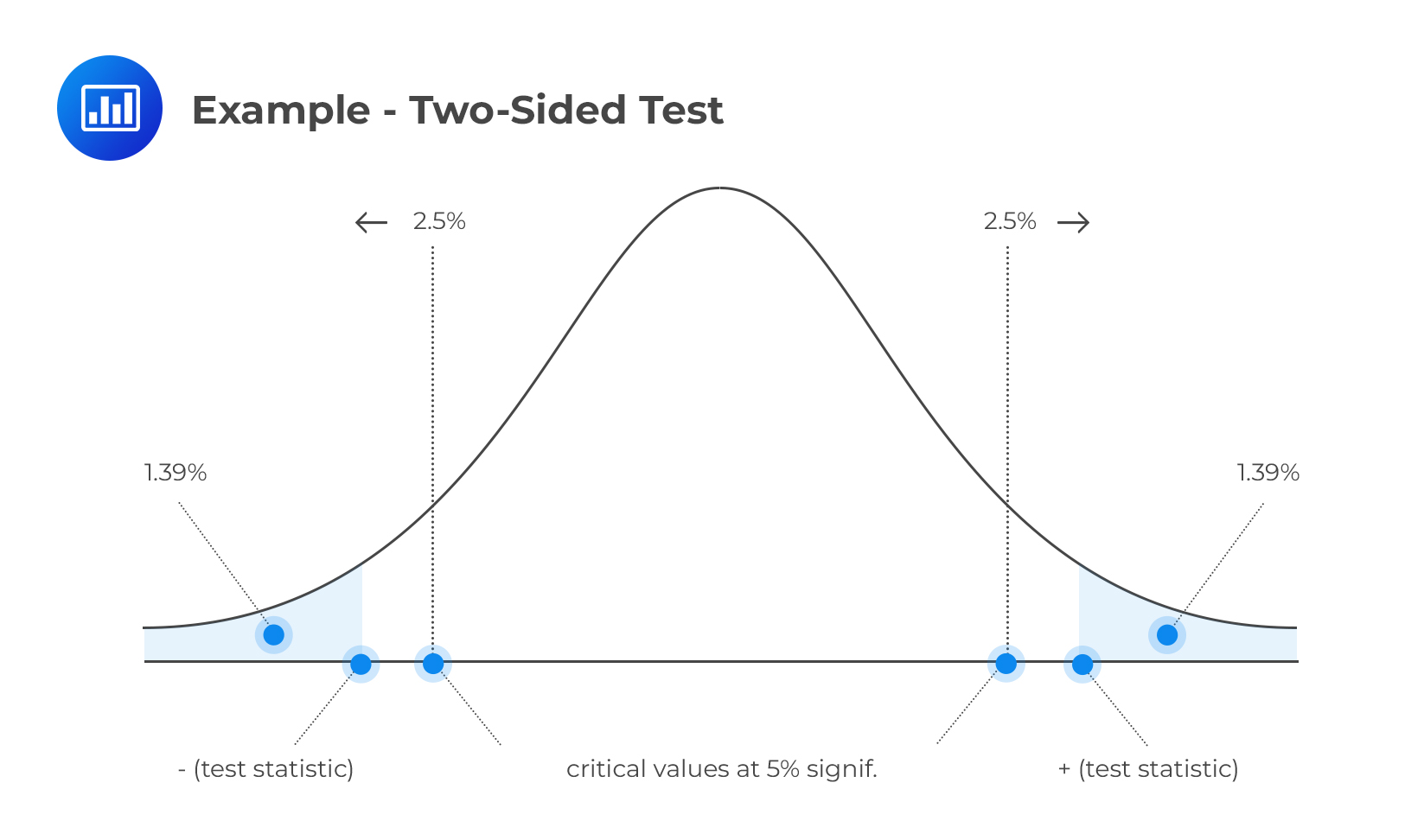
H0: μ = μ0 vs. H1: μ ≠ μ0
She obtains a test statistic of 2.2. Given a 5% significance level, determine and interpret the p-value
Solution
$$ \text{P-value}=2P(Z>2.2)=2[1–P(Z≤2.2)] =1.39\%×2=2.78\%$$
(We have multiplied by two since this is a two-tailed test)
 Interpretation
The p-value (2.78%) is less than the level of significance (5%). Therefore, we have sufficient evidence to reject H0. In fact, the evidence is so strong that we would also reject H0 at significance levels of 4% and 3%. However, at significance levels of 2% or 1%, we would not reject H0 since the p-value surpasses these values.
It’s common for analysts to be interested in establishing whether there exists a significant difference between the means of two different populations. For instance, they might want to know whether the average returns for two subsidiaries of a given company exhibit significant differences.
Now, consider a bivariate random variable:
$$W_i=[X_i,Y_i]$$
Assume that the components \(X_i\) and \(Y_i\)are both iid and are correlated. That is:
\(\text{Corr} (X_i,Y_i )≠0\)
Now, suppose that we want to test the hypothesis that:
$$H_0:μ_X=μ_Y$$
$$H_1:μ_X≠μ_Y$$
In other words, we want to test whether the constituent random variables have equal means. Note that the hypothesis statement above can be written as:
$$H_0:μ_X-μ_Y=0$$
$$H_1:μ_X-μ_Y≠0$$
To execute this test, consider the variable:
$$Z_i=X_i-Y_i$$
Therefore, considering the above random variable, if the null hypothesis is correct then,
$$E(Z_i)=E(X_i)-E(Y_i)=μ_X-μ_Y=0$$
Intuitively, this can be considered as a standard hypothesis test of
H0: μZ =0 vs. H1: μZ ≠ 0.
The tests statistic is given by:
$$T=\frac{\hat{\mu}_z}{\sqrt{\frac{\hat{\sigma}^2_z}{n}}} \sim N(0,1)$$
Note that the test statistic formula accounts for the correction between \(X_i \) and \(Y_i\). It is easy to see that:
$$V(Z_i)=V(X_i )+V(Y_i)-2COV(X_i, Y_i)$$
Which can be denoted as:
$$\hat{\sigma}^2_z =\hat{\sigma}^2_X +\hat{\sigma}^2_Y – 2{\sigma}_{XY}$$
$$ \hat{\mu}_z ={\mu}_X-{\mu}_Y $$
And thus the test statistic formula can be written as:
$$T=\frac{{\mu}_X -{\mu}_Y}{\sqrt{\frac{\hat{\sigma}^2_X +\hat{\sigma}^2_Y – 2{\sigma}_{XY}}{n}}}$$
This formula indicates that correlation plays a crucial role in determining the magnitude of the test statistic.
Another special case of the test statistic is when \(X_i\), and \(Y_i\) are iid and independent. The test statistic is given by:
$$T=\frac{{\mu}_X -{\mu}_Y}{\sqrt{\frac{\hat{\sigma}^2_X}{n_X}+\frac{\hat{\sigma}^2_Y}{n_Y}}}$$
Where \(n_X\) and \(n_Y\) are the sample sizes of \(X_i\), and \(Y_i\) respectively.
An investment analyst wants to test whether there is a significant difference between the means of the two portfolios at a 95% level. The first portfolio X consists of 30 government-issued bonds and has a mean of 10% and a standard deviation of 2%. The second portfolio Y consists of 30 private bonds with a mean of 14% and a standard deviation of 3%. The correlation between the two portfolios is 0.7. Calculate the null hypothesis and state whether the null hypothesis is rejected or otherwise.
Solution
The hypothesis statement is given by:
H0: μX – μY=0 vs. H1: μX – μY ≠ 0.
Note that this is a two-tailed test. At 95% level, the test size is α=5% and thus the critical value \(C_α=±1.96\).
Recall that:
$$Cov(X, Y)=σ_{XY}=ρ_{XY} σ_X σ_Y$$
Where ρ_XY is the correlation coefficient between X and Y.
Now the test statistic is given by:
$$T=\frac{{\mu}_X -{\mu}_Y}{\sqrt{\frac{\hat{\sigma}^2_X +\hat{\sigma}^2_Y – 2{\sigma}_{XY}}{n}}}=\frac{{\mu}_X -{\mu}_Y}{\sqrt{\frac{\hat{\sigma}^2_X +\hat{\sigma}^2_Y – 2{\rho}_{XY} {\sigma}_X {\sigma}_Y}{n}}}$$
$$=\frac{0.10-0.14}{\sqrt{\frac{0.02^2 +0.03^2-2\times 0.7 \times 0.02 \times 0.03}{30}}}=-10.215$$
The test statistic is far much less than -1.96. Therefore the null hypothesis is rejected at a 95% level.
Multiple testing occurs when multiple multiple hypothesis tests are conducted on the same data set. The reuse of data results in spurious results and unreliable conclusions that do not hold up to scrutiny. The fundamental problem with multiple testing is that the test size (i.e., the probability that a true null is rejected) is only applicable for a single test. However, repeated testing creates test sizes that are much larger than the assumed size of alpha and therefore increases the probability of a Type I error.
Some control methods have been developed to combat multiple testing. These include Bonferroni correction, the False Discovery Rate (FDR), and Familywise Error Rate (FWER).
Practice Question
An experiment was done to find out the number of hours that candidates spend preparing for the FRM part 1 exam. For a sample of 10 students, the average study time was found to be 312.7 hours, with a standard deviation of 7.2 hours. What is the 95% confidence interval for the mean study time of all candidates?
A. [307.5, 317.9]
B. [310, 317]
C. [300, 317]
D. [307.5, 312.2]
The correct answer is A.
To calculate the 95% confidence interval for the mean study time of all candidates, we can use the formula for the confidence interval when the population variance is unknown:
\[\text{Confidence Interval} = \bar{X} \pm t_{1-\frac{\alpha}{2}} \times \frac{s}{\sqrt{n}}\]
Where:
- \(\bar{X}\) is the sample mean
- \(t_{1-\frac{\alpha}{2}}\) is the t-score corresponding to the desired confidence level and degrees of freedom
- \(s\) is the sample standard deviation
- \(n\) is the sample size
In this case:
- \(\bar{X} = 312.7\) hours (the average study time)
- \(s = 7.2\) hours (the standard deviation of study time)
- \(n = 10\) students (the sample size)
To find the t-score (\(t_{1-\frac{\alpha}{2}}\)), we look at the t-table for the 95% confidence level (which corresponds to \(\alpha = 0.05\)) and 9 degrees of freedom (\(n – 1 = 10 – 1 = 9\)). The t-score is 2.262.
Now, we can plug these values into the confidence interval formula:
\[\text{Confidence Interval} = 312.7 \pm 2.262 \times \frac{7.2}{\sqrt{10}}\]
Calculating the margin of error:
\[\text{Margin of Error} = 2.262 \times \frac{7.2}{\sqrt{10}} \approx 5.2\]
So the confidence interval is:
\[\text{Confidence Interval} = 312.7 \pm 5.2 = [307.5, 317.9]\]
Therefore, the 95% confidence interval for the mean study time of all candidates is [307.5, 317.9] hours.
Offered by AnalystPrep


