


Machine Learning Methods
After completing this reading, you should be able to: Discuss the philosophical and... Read More

After completing this reading, you should be able to:
Economic capital of a bank is the approximate amount of capital that the bank requires to absorb the losses from the loan portfolios. In other words, it is the cushion that a bank estimates it will need in order to remain solvent.
Regulatory capital is the amount of capital the regulators require the banks to maintain. For instance, the Global bank requirements are determined by the Basel Committee on Banking Supervision (BCBS) based in Switzerland. Supervisors then implement the BCBS requirements in each country.
Banks also have what is called debt capital, funded by bondholders. In case the incurred losses deplete the equity capital, the debt holders should incur losses before the depositors.
The equity capital is described as “going concern capital” because the bank is solvent if its capital is positive. On the other hand, the debt capital is described as the “gone concern capital” because it acts as a cushion to the depositors when the bank becomes insolvent (no longer a going concern).
Banks face many risks through their transactions, which need to be quantified. Credit risk is a primary risk that the banks have concentrated since the inception of the banking industry. It is majorly explained by the fact that the banks’ activities mainly involve taking deposits and making loans. The loans made are predisposed to some level of default of risk and hence some level of credit loss (credit risk).
Credit risk is quantified using different models. This chapter discusses three models:
The defaults among bank borrowers are not independent because if this would have been the case, then we would expect a similar default rate each year.
In reality, loans do not default independently of one another. Instead, there are good and bad years for defaults.
Among the reasons why companies do not default independently is the economy. Risks associated with the economy are usually systematic and non-diversifiable, which cannot be diversified away by banks and bondholders. Good economic conditions immediately before and during the year lower the probability of default for all companies. On the other hand, bad economic conditions immediately before and during the year raise the probability of default for all companies during the year.
Another reason why companies do not default independently of each other is the credit contagion. Credit contagion is the process by which a problem in one company spreads to other companies as well. To illustrate this, consider three companies X, Y, and Z. Suppose that company X purchases goods from company Y and that in turn, Company Y buys goods from Company Z. Now, if Company X goes bankrupt, Company Y will suffer and it may even go bankrupt depending on the volume of transactions between the two companies. This could lead to Company Z failing even though it had no direct exposure to Company X.
The importance of credit contagion to non-financial companies is still a matter of discussion. The banking regulators are concerned, however, about the potential for credit contagion. Such risks are called systemic risks. In the event that Bank X fails, bank Y will suffer a huge loss as a result of the transactions it has with bank X. Bank Y, may thus default. Bank Z will be affected as well if it has outstanding transactions with Bank Y.
The expected loss, EL, is the average credit loss that we would expect from an exposure or a portfolio over a given period. It is the anticipated deterioration in the value of a risky asset. In mathematical terms,
$$ \text{EL}=\text{EA}\times\text{PD}\times\text{LGD} $$
Where:
\(\text{EA}=\) exposure amount also known as exposure at default (EAD).
\(\text{PD}=\) probability of default.
\(\text{LGD}=\) loss given default also known as loss rate.
Credit loss levels are not constant but rather fluctuate from year to year. The expected loss represents the anticipated average loss that can be statistically determined. Businesses will typically have a budget for the EL and try to bear the losses as part of the standard operating cash flows.
Exam tip: The expected loss of a portfolio is equal to the summation of expected losses of personal losses.
$$ { \text{EL} }_{ \text{P} }=\sum { { \text{EA} }_{ \text{i} } } \times { \text{PD} }_{ \text{i} }\times \text{LGD}_{ \text{i} } $$
A Canadian bank recently disbursed a CAD 2 million loan, of which CAD 1.6 million is currently outstanding. According to the bank’s internal rating model, the beneficiary has a 1% chance of defaulting over the next year. In case that happens, the estimated loss rate is 30%. The probability of default and the loss rate have standard deviations of 6% and 20%, respectively. Determine the expected loss figures for the bank.
$$ EL =EA×PD×LR $$
Where:
\(EA\) = CAD 1,600,000
\(PD\) = 1%
\(LR\) = 30%
Thus,
$$ \text{EL}=1,600,000\times0.01\times0.3=\text{CAD } 4,800 $$
Unexpected loss is the average total loss over and above the expected loss.
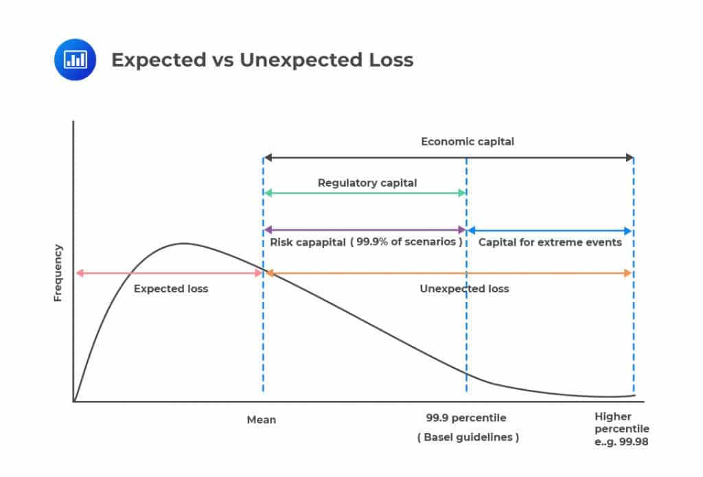 It is the variation in the expected loss. It is calculated as the standard deviation from the mean at a certain confidence level.
Let \({\text{UH}}_{\text{L}}\) denote the unexpected loss at the horizon for asset value \({\text{V}}_{\text{H}}\). Then,
$$ {\text{UH}}_{\text{L}} \equiv \sqrt{\left(\text{var}\left(\text{VH}\right) \right)} $$
You will usually apply the following formula to determine the value of the unexpected loss:
$$ \text{UL}=\text{EA}\times\sqrt{\text{PD}\times{{ \sigma }_{ \text{LR} }^{ 2 }+{ \text{LR} }^{ 2 }\times{ \sigma }_{ \text{PD} }^{ 2 }}} $$
Where
$$ { \sigma }_{ \text{PD} }^{ 2 }=\text{PD}\times\left(1-\text{PD}\right) $$
Given that a bank has n loans, define the following quantities:
\({\text{L}}_{\text{i}}\) – the amount borrowed in the ith assumed to be constant throughout the year.
\({\text{p}}_{\text{i}}\) – the probability of the default for the ith loan
\({\text{R}}_{\text{i}}\) – the recovery rate in the event of the default by the ith loan
\({\text{p}}_{\text{ij}}\) – the correlation between losses on the ith and jth loan
\({\sigma}_{\text{i}}\) – the standard deviation of loss on the ith and jth loan
\({\sigma}_{\text{p}}\) – the standard deviation of loss from the portfolio
\(\text a\) – the standard deviation of portfolio loss as a fraction of the size of the portfolio
If the ith loan defaults, the loss is given by:
$$ {\text{L}}_{\text{i}} \left(1-{\text{R}}_{\text{i}}\right) $$
Intuitively, the probability distribution for the loss from the ith loan is made of a probability \(p_i\) that there will be a loss of this amount and the probability \(1-p_i\) that there is no loss, which is typically a binomial distribution. Therefore, we can present the mean and the standard deviation of the loss.
The mean of the loss is given by:
$$ {\text{p}}_{\text{i}}\times{\text{L}}_{\text{i}} \left(1-{\text{R}}_{\text{i}}\right)+\left(1-{\text{p}}_{\text{i}}\right)\times0={\text{p}}_{\text{i}}{\text{L}}_{\text{i}}\left(1-{\text{R}}_{\text{i}}\right) $$
Now, recall that for a random variable X, the variance is defined as:
$$ { \sigma }_{ \text{x} }=E\left({\text{x}}^{2}\right)-[E\left({\text{x}}\right)]^2 $$
Where E denotes the expectation. Intuitively,
$$ { \sigma }_{ \text{i} }^{ 2 }={\text{E}}\left({\text{Loss}}^{2}\right)-\left[\text{E}\left({\text{Loss}}\right)\right]^{2} $$
This follows immediately that:
$$ \begin{align*} { \sigma }_{ \text{i} }^{ 2 }={ \text{p} }_{ \text{i} }{ \left[ { \text{L} }_{ \text{i} }\left( 1-{ \text{R} }_{ \text{i} } \right) \right] }^{ 2 }-{ \left[ { \text{p} }_{ \text{i} }{ \text{L} }_{ \text{i} }\left( 1-{ \text{R} }_{ \text{i} } \right) \right] }^{ 2 }=\left( { \text{p} }_{ \text{i} }-{ \text{p} }_{ { \text{i} } }^{ 2 } \right) { \left[ { \text{L} }_{ \text{i} }\left( 1-{ \text{R} }_{ \text{i} } \right) \right] }^{ 2 } \end{align*} $$
So that the standard deviation of the loss is given by:
$$ { \sigma }_{ \text{i} }=\sqrt { { \text{p} }_{ \text{i} }-{ \text{p} }_{ \text{i} }^{ 2 } } \left[ { \text{L} }_{ \text{i} }\left( 1-{ \text{R} }_{ \text{i} } \right) \right] $$
Note that we can also calculate the standard deviation of the loan portfolio from the losses on the individual loans. It is given by:
$$ { \sigma }_{ { \text{P} } }^{ 2 }=\sum _{ \text{i}=1 }^{ \text{n} }{ \sum _{ \text{j}=1 }^{ \text{n} }{ { \text{p} }_{ \text{ij} } } { \sigma }_{ \text{i} }{ \sigma }_{ \text{j} } } ……………Eq1 $$
Now, the standard deviation expressed as the percentage of the size of the portfolio is
$$ \alpha =\cfrac { \sqrt { \sum _{ \text{i}=1 }^{ \text{n} }{ \sum _{ \text{j}=1 }^{ \text{n} }{ { \text{p} }_{ \text{ij} } } { \sigma }_{ \text{i} }{ \sigma }_{ \text{j} } } } }{ \sum _{ \text{i}=1 }^{ \text{n} }{ \text{L}_{ \text{i} } } } ……………..Eq2 $$
Assume that all loans have the same principal L, all recovery rate R are equal, and all default probabilities are equal and denoted by \(P\), and the correlation coefficient is defined as:
$$ { \rho }_{ \text{ij} }=\begin{cases} 1\quad \text{when}\quad { i }={ j } \\ { \rho }\quad { \text{when} }\quad { i }\neq { j } \end{cases} $$
Where ρ is constant.
Therefore, the standard deviation of the loss from loan i is the same for all i so that the common standard deviation denoted by σ is given by:
$$ {\sigma}=\sqrt { { \text{p} }-{ \text{p} }^{ 2 } } \left[ { \text{L} }\left( 1-{ \text{R} } \right) \right] $$
Therefore, Eq1 reduces to:
$$ { \sigma }_{ { \text{P} } }^{ 2 }=\text{n}{ \sigma }^{ 2 }+\text{n}\left( \text{n}-1 \right) \rho { \sigma }^{ 2 } $$
Also, the standard deviation of the loss from the loan portfolio as a percentage of its size (Eq2) reduces to:
$$ \alpha =\cfrac { { \sigma }_{ { \text{P} } } }{ \text{nL} } =\cfrac { \sigma \sqrt { 1+\left( \text{n}-1 \right) \rho } }{ \text{L}\sqrt { \text{n} } } $$
The bank of Baroda has a portfolio consisting of 10,000 loans, each loan amounting to $2 million and has a 1% probability of default over the following year. The recovery rate is 40%, and the correlation coefficient is 0.1. Calculate \(\alpha\), the standard deviation of the loss from the loan portfolio as a percentage of its size?
The \(\alpha\) parameter is given by:
$$ \alpha =\cfrac { \sigma \sqrt { 1+\left( \text{n}-1 \right) \rho } }{ \text{L}\sqrt { \text{n} } } $$
For this case,
L = $2 million
P=0.01
ρ = 0.1
n = 10,000
R = 0.4
$$ \begin{align*} {\sigma}&=\sqrt { { \text{p} }-{ \text{p} }^{ 2 } } \left[ { \text{L} }\left( 1-{ \text{R} } \right) \right] \\ &=\sqrt{0.01-{0.01}^{2}}\left[ { 2 }\left( 1-{ 0.4 } \right) \right]=0.1194 \end{align*} $$
Therefore,
$$ \alpha = \cfrac { 0.1194\sqrt { 1+\left( 10,000-1 \right) \times 0.1 } }{ 2\times \sqrt { 10,000 } } =0.01889 $$
A Gaussian copula maps the marginal distribution of each variable to the standard normal distribution, which, by definition, has a mean of zero and a standard deviation of one. Copula correlation models create a joint probability distribution for two or more variables while still preserving their marginal distributions. The joint probability of the variables of interest is implicitly defined by mapping them to other variables whose distribution properties are known.
We can demonstrate how Gaussian copulas work using a simple example:
Let us define two variables \({\text{V}}_{1}\) and \({\text{V}}_{2}\) that have unknown distributions and unique marginal distributions. \({\text{V}}_{1}\) and \({\text{V}}_{2}\) are mapped into new variables \({\text{U}}_{1}\) and \({\text{U}}_{2}\), respectively, that have standard normal distributions. The mapping is done on a percentile-to-percentile basis to create a Gaussian copula.
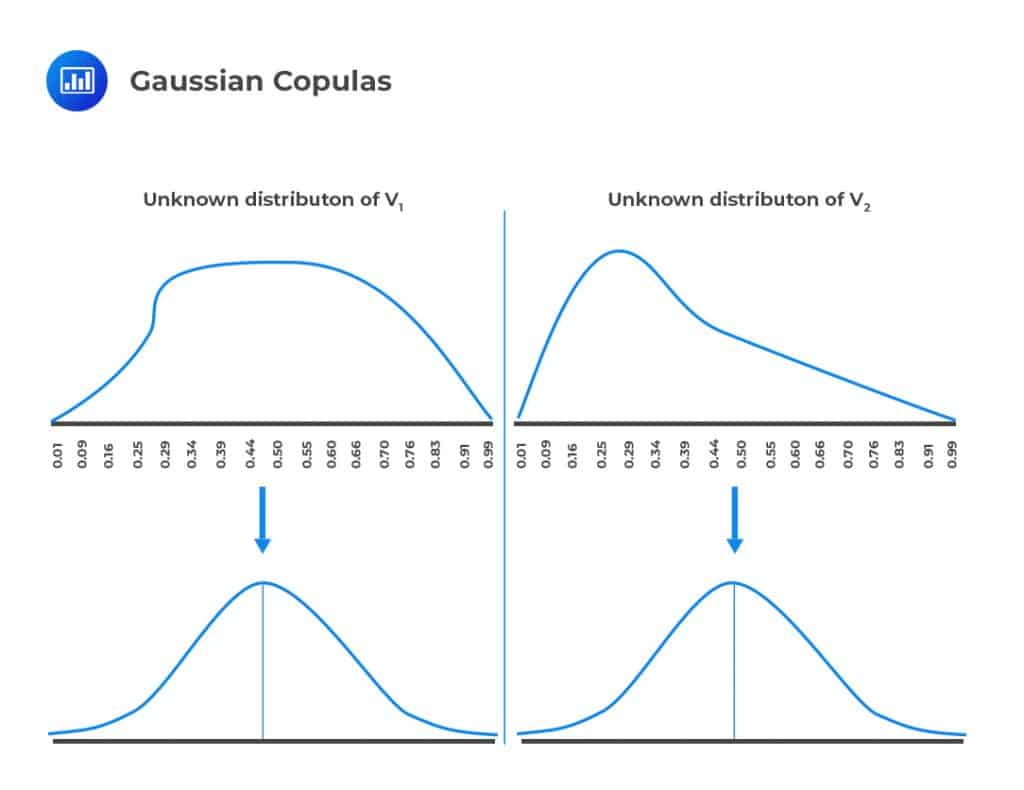 For example, the one-percentile point of the \({\text{V}}_{1}\) distribution is mapped to the one-percentile point of the \({\text{U}}_{1}\) distribution. Similarly, the 50-percentile point of the \({\text{V}}_{1}\) distribution is mapped to the 50-percentile point of the \({\text{U}}_{1}\) distribution.
Before mapping variables \({\text{V}}_{1}\) and \({\text{V}}_{2}\) to the normal distribution, it is very difficult to define a relationship between them since their marginal distributions are unknown and are pretty much incomprehensible structures. Once they have been mapped to the standard normal distribution as new variables \({\text{U}}_{1}\) and \({\text{U}}_{2}\), respectively, we can now define a relationship between them since the standard normal distribution has a known structure. The Gaussian copula, therefore, helps us to define a correlation between variables when it is not possible to define a correlation directly.
Assume now that we have many variables \({\text{V}}_{\text{i}}\) for all i=1,2,…,n for which each of the \({\text{V}}_{\text{i}}\) can be mapped to a standard normal distribution \({\text{U}}_{\text{i}}\). The main challenge that remains is to define the correlation between \({\text{U}}_{\text{i}}\) distributions because the presence of many unique distributions means that we have to specify numerous correlation parameters. To address this issue, we use the one-factor model.
The one-factor model is defined as:
$$ {\text{U}}_{\text{i}}= {\text a}_{\text{i}}{\text{F}}+\sqrt{1-{ \text a }_{ { \text{i} } }^{ 2 }}{\text{Z}}_{\text{i}} $$
Where F is a common factor for all \({\text{U}}_{\text{i}}\) and \({\text{Z}}_{\text{i}}\) is a component of \({\text{U}}_{\text{i}}\) that is unrelated to the factor F and uncorrelated to each other. The \(\text a_{\text i}\) are the parameter values that lie between -1 and +1, that is \(\text a_{\text i} \in [-1,+1]\).
The variables F and \({\text{Z}}_{\text{i}}\) have the standard normal distributions, that is, \(F \sim N(0,1)\) and \({\text{Z}}_{\text{i}} \sim N(0,1)\). Therefore, \({\text{U}}_{\text{i}}\) is a sum of two independent normal distributions, and it is, therefore, a normal variable with a mean of 0 and a standard deviation of 1. The variance of \({\text{U}}_{\text{i}}\) is 1 since F and \({\text{Z}}_{\text{i}}\) are uncorrelated so that:
$$ \begin{align*} \text{Var}\left( { \text{U} }_{ \text{i} } \right) &=\text{Var}\left[ {\text a}_{\text{i}}{\text{F}}+\sqrt{1-{ \text a }_{ { \text{i} } }^{ 2 }}{\text{Z}}_{\text{i}} \right] \\ &={ \text a }_{ \text{i} }^{ 2 }\text{Var}\left( \text{F} \right) +{ \left( \sqrt { 1-{ \text a }_{ \text{i} }^{2} } \right) }^{ 2 }\text{Var}\left( { { \text{Z} } }_{ { \text{i} } } \right) \\ &={ \text a }_{ \text{i} }^{ 2 }.1+{ \left( \sqrt { 1-{ \text a }_{ \text{i} }^{2} } \right) }^{ 2 }.1={ \text a }_{ \text{i} }^{ 2 }+1-{ \text a }_{ \text{i} }^{ 2 }=1 \end{align*} $$
Note that we are summing the variances of two uncorrelated variables.
So in a nutshell, the one-factor model takes one standard normally distributed variable \({\text{U}}_{\text{i}}\) and defines it in relation to two other variables, which are both standard normally distributed. The factor \(F\) affects across all \({\text{U}}_{\text{i}}\) but factor \({\text{Z}}_{\text{i}}\) affects only \({\text{U}}_{\text{i}}\).
The coefficient of correlation between \({\text{U}}_{\text{i}}\) and \({\text{U}}_{\text{j}}\) comes in as a result of their dependence on the common factor F and thus is \({\text{a}}_{\text{i}}\) \({\text{a}}_{\text{j}}\). The correlation coefficient between \({\text{U}}_{\text{i}}\) and \({\text{U}}_{\text{j}}\) is defined from the basic statistics as
$$ \begin{align*} { \rho }_{ { \text{U} }_{ \text{i} },{ \text{U} }_{ \text{j} } }=\cfrac { \text{E}\left( { \text{U} }_{ \text{i} }{ \text{U} }_{ \text{j} } \right) -\text{E}\left( { \text{U} }_{ \text{i} } \right) \text{E}\left( { \text{U} }_{ \text{j} } \right) }{ { \sigma }_{ { { \text{U} } }_{ { \text{i} } } }{ \sigma }_{ { { \text{U} } }_{ \text{j} } } } \end{align*} $$
But \(\text{E}\left( { \text{U} }_{ \text{i} }\right)\)=\(\text{E}\left( { \text{U} }_{ \text{j} }\right)\)=0 and \({ \sigma }_{ { \text{U} }_{ \text{i} }}={ \sigma }_{ { \text{U} }_{ \text{j} }}=1\) and thus the above equation reduces to
$$ { \rho }_{ { \text{U} }_{ \text{i} },{ \text{U} }_{ \text{j} } }=\cfrac { \text{E}\left( { \text{U} }_{ \text{i} }{ \text{U} }_{ \text{j} } \right) -0 }{ 1 } =\text{E}\left( { \text{U} }_{ \text{i} }{ \text{U} }_{ \text{j} } \right) $$
Now,
$$ \begin{align*} \text{E}\left( { \text{U} }_{ \text{i} }{ \text{U} }_{ \text{j} } \right) =\text{E}\left[ \left( { \text a }_{ { \text{i} } }{ { \text{F} } }+\sqrt { 1-{ \text a }_{ { { \text{i} } } }^{ 2 } } { { \text{Z} } }_{ { \text{i} } } \right) \left( { \text a }_{ { \text{j} } }{ { \text{F} } }+\sqrt { 1-{ \text a }_{ { { \text{j} } } }^{ 2 } } { { \text{Z} } }_{ { \text{j} } } \right) \right] \end{align*} $$
But \(F\) is uncorrelated with all \({ { \text{Z} } }_{ { \text{i} } }\) and \({ { \text{Z} } }_{ { \text{i} } }\) is uncorrelated with \({ { \text{Z} } }_{ { \text{j} } }\) so that
$$ \text{E}\left( { \text{FZ} }_{ \text{i} } \right)=\text{E}\left( { \text{FZ} }_{ \text{j} } \right)=\text{E}\left( { \text{Z} }_{ \text{i} }{ \text{Z} }_{ \text{j} } \right)=0 $$
And the above equation reduces to:
$$ \begin{align*} \text{E}\left( { \text{U} }_{ \text{i} }{ \text{U} }_{ \text{j} } \right) &= \text{E}\left( { \text a }_{ \text{i} },{ \text a }_{ \text{j} }{\text{F}}^{2}\right)={ \text a }_{ \text{i} },{ \text a }_{ \text{j} }{\text{E}}\left({\text{F}}^{2}\right)={ \text a }_{ \text{i} },{ \text a }_{ \text{j} }.1={ \text a }_{ \text{i} },{ \text a }_{ \text{j} } \\ &\therefore { \rho }_{ { \text{U} }_{ \text{i} },{ \text{U} }_{ \text{j} } } ={ \text a }_{ \text{i} }{ \text a }_{ \text{j} } \end{align*} $$
Note that the immediate result stems from the fact that \(\text E(\text F^2 )=1\) because F is a standard normal variable, \(\text F \sim \text N(0,1)\) so that:
$$ \begin{align*} {\text{E}}\left({\text{F}}^{2}\right)-\left[{\text{E}}\left({\text{F}}\right)\right]^{2}&= \text {Var}\left({\text{F}}\right)=1 \\ \Rightarrow {\text{E}}\left({\text{F}}^{2}\right)-\left[0\right]^{2}&=1 \\ \therefore {\text{E}}\left({\text{F}}^{2}\right)&=1 \end{align*} $$
A notable example of a one-factor model is the capital asset pricing model (CAPM). In CAPM, the correlation coefficient between two assets is assumed to arise from the dependence on the common factor – the return from the market index. However, CAPM is significantly palatable since it specifies the correlation between the returns of the different assets.
The Vasicek model uses the Gaussian copula model to define the correlation between the defaults when determining the capital for loan portfolios. The Vasicek model has an advantage over the standard deviation of the loss from the loan portfolio as a percentage of its size, α in that the unexpected loss can be determined analytically.
Now, assume that the probability of default (PD) is the same for all firms in a huge portfolio so that the PD for a company i for one year is mapped to a standard normal \({ \text{U} }_{ \text{i} }\) as described earlier.
Consider the following figure below:
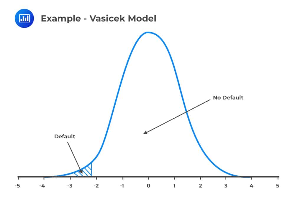 The values at the further left (shaded region) tail of this standard normal distribution is the distribution of the default, while the rest is the distribution of no default.
Mathematically, a firm i defaults if:
$$ { \text{U} }_{ \text{i} }\le { \text{N} }^{ -1 }\left( \text{PD} \right) $$
Where \(\text N^{-1}\) is the inverse of the inverse cumulative normal distribution. That is if the probability of default for the loan portfolio of a bank is 1%, then the bank defaults if:
$$ { \text{U} }_{ \text{i} }\le { \text{N} }^{ -1 }\left( 0.01 \right)=-2.326 $$
$$\small{\begin{array}{l|cccccccccc}
\textbf{z} & \textbf{0.00} & \textbf{0.01} & \textbf{0.02} & \textbf{0.03} & \textbf{0.04} & \textbf{0.05} & \textbf{0.06} & \textbf{0.07} & \textbf{0.08} & \textbf{0.09} \\\hline
\textbf{-3.0} & 0.0013 & 0.0013 & 0.0013 & 0.0012 & 0.0012 & 0.0011 & 0.0011 & 0.0011 & 0.0010 & 0.0010 \\
\textbf{-2.9} & 0.0019 & 0.0018 & 0.0018 & 0.0017 & 0.0016 & 0.0016 & 0.0015 & 0.0015 & 0.0014 & 0.0014 \\
\textbf{-2.8} & 0.0026 & 0.0025 & 0.0024 & 0.0023 & 0.0023 & 0.0022 & 0.0021 & 0.0021 & 0.0020 & 0.0019 \\
\textbf{-2.7} & 0.0035 & 0.0034 & 0.0033 & 0.0032 & 0.0031 & 0.0030 & 0.0029 & 0.0028 & 0.0027 & 0.0026 \\
\textbf{-2.6} & 0.0047 & 0.0045 & 0.0044 & 0.0043 & 0.0041 & 0.0040 & 0.0039 & 0.0038 & 0.0037 & 0.0036 \\
\textbf{-2.5} & 0.0062 & 0.0060 & 0.0059 & 0.0057 & 0.0055 & 0.0054 & 0.0052 & 0.0051 & 0.0049 & 0.0048 \\
\textbf{-2.4} & 0.0082 & 0.0080 & 0.0078 & 0.0075 & 0.0073 & 0.0071 & 0.0069 & 0.0068 & 0.0066 & 0.0064 \\
\textbf{-2.3} & 0.0107 & 0.0104 & 0.0102 & \textbf{0.0099} & 0.0096 & 0.0094 & 0.0091 & 0.0089 & 0.0087 & 0.0084 \\
\textbf{-2.2} & 0.0139 & 0.0136 & 0.0132 & 0.0129 & 0.0125 & 0.0122 & 0.0119 & 0.0116 & 0.0113 & 0.0110 \\
\textbf{-2.1} & 0.0179 & 0.0174 & 0.0170 & 0.0166 & 0.0162 & 0.0158 & 0.0154 & 0.0150 & 0.0146 & 0.0143 \\
\textbf{-2.0} & 0.0228 & 0.0222 & 0.0217 & 0.0212 & 0.0207 & 0.0202 & 0.0197 & 0.0192 & 0.0188 & 0.0183 \\
\textbf{-1.9} & 0.0287 & 0.0281 & 0.0274 & 0.0268 & 0.0262 & 0.0256 & 0.0250 & 0.0244 & 0.0239 & 0.0233 \\
\textbf{-1.8} & 0.0359 & 0.0351 & 0.0344 & 0.0336 & 0.0329 & 0.0322 & 0.0314 & 0.0307 & 0.0301 & 0.0294 \\
\textbf{-1.7} & 0.0446 & 0.0436 & 0.0427 & 0.0418 & 0.0409 & 0.0401 & 0.0392 & 0.0384 & 0.0375 & 0.0367 \\
\textbf{-1.6} & 0.0548 & 0.0537 & 0.0526 & 0.0516 & 0.0505 & 0.0495 & 0.0485 & 0.0475 & 0.0465 & 0.0455 \\
\textbf{-1.5} & 0.0668 & 0.0655 & 0.0643 & 0.0630 & 0.0618 & 0.0606 & 0.0594 & 0.0582 & 0.0571 & 0.0559 \\
\textbf{-1.4} & 0.0808 & 0.0793 & 0.0778 & 0.0764 & 0.0749 & 0.0735 & 0.0721 & 0.0708 & 0.0694 & 0.0681 \\
\textbf{-1.3} & 0.0968 & 0.0951 & 0.0934 & 0.0918 & 0.0901 & 0.0885 & 0.0869 & 0.0853 & 0.0838 & 0.0823 \\
\textbf{-1.2} & 0.1151 & 0.1131 & 0.1112 & 0.1093 & 0.1075 & 0.1056 & 0.1038 & 0.1020 & 0.1003 & 0.0985 \\
\textbf{-1.1} & 0.1357 & 0.1335 & 0.1314 & 0.1292 & 0.1271 & 0.1251 & 0.1230 & 0.1210 & 0.1190 & 0.1170 \\
\textbf{-1.0} & 0.1587 & 0.1562 & 0.1539 & 0.1515 & 0.1492 & 0.1469 & 0.1446 & 0.1423 & 0.1401 & 0.1379 \\
\textbf{-0.9} & 0.1841 & 0.1814 & 0.1788 & 0.1762 & 0.1736 & 0.1711 & 0.1685 & 0.1660 & 0.1635 & 0.1611 \\
\textbf{-0.8} & 0.2119 & 0.2090 & 0.2061 & 0.2033 & 0.2005 & 0.1977 & 0.1949 & 0.1922 & 0.1894 & 0.1867 \\
\textbf{-0.7} & 0.2420 & 0.2389 & 0.2358 & 0.2327 & 0.2296 & 0.2266 & 0.2236 & 0.2206 & 0.2177 & 0.2148 \\
\textbf{-0.6} & 0.2743 & 0.2709 & 0.2676 & 0.2643 & 0.2611 & 0.2578 & 0.2546 & 0.2514 & 0.2483 & 0.2451 \\
\textbf{-0.5} & 0.3085 & 0.3050 & 0.3015 & 0.2981 & 0.2946 & 0.2912 & 0.2877 & 0.2843 & 0.2810 & 0.2776 \\
\textbf{-0.4} & 0.3446 & 0.3409 & 0.3372 & 0.3336 & 0.3300 & 0.3264 & 0.3228 & 0.3192 & 0.3156 & 0.3121 \\
\textbf{-0.3} & 0.3821 & 0.3783 & 0.3745 & 0.3707 & 0.3669 & 0.3632 & 0.3594 & 0.3557 & 0.3520 & 0.3483 \\
\textbf{-0.2} & 0.4207 & 0.4168 & 0.4129 & 0.4090 & 0.4052 & 0.4013 & 0.3974 & 0.3936 & 0.3897 & 0.3859 \\
\textbf{-0.1} & 0.4602 & 0.4562 & 0.4522 & 0.4483 & 0.4443 & 0.4404 & 0.4364 & 0.4325 & 0.4286 & 0.4247 \\
\textbf{-0.0} & 0.5000 & 0.4960 & 0.4920 & 0.4880 & 0.4840 & 0.4801 & 0.4761 & 0.4721 & 0.4681 & 0.4641
\end{array}}$$
This can be stated as a bank defaults if:
$$ { \text{U} }_{ \text{i} }\in \left( -\infty ,-2.326 \right) $$
And no default if:
$$ { \text{U} }_{ \text{i} } \in \left( -2.326 ,\infty \right) $$
Recall that the one-factor model is given by:
$$ { \text{U} }_{ \text{i} }={ \text a }_{ \text{i} }{\text{F}}+\sqrt { 1-{ \text a }_{ { { \text{i} } } }^{ 2 } } { { \text{Z} } }_{ { \text{i} } } $$
To make the model more palatable, \(\text a_{\text i}\)’s are assumed to be equal for all i so that \({ \text{a} }_{ \text{i} }=\text a\) and thus, the one-factor model is rewritten as:
$$ { \text{U} }_{ \text{i} }={\text a \text{F}}+\sqrt { 1-{ \text a }^{ 2 } } { { \text{Z} } }_{ { \text{i} } } $$
Thus the correlation between each pair of \({\text{U}}_{\text{i}}\)’s is:
$$ { \rho }_{ { { \text{U} } }_{ { \text{i} } },{ { \text{U} } }_{ { \text{j} } } }={ \text a }_{ { { \text{i} } } }{ \text a }_{ { { \text{j} } } }=\text a .\text a ={ \text a }^{ 2 } $$
Now, the factor F can be taken as an index of the recent economic health. That is, if the F is high the doing economy is healthy implying that \({\text{U}}_{\text{i}}\) is high, making the default relatively low. Otherwise, if F is relatively low, then \({\text{U}}_{\text{i}}\) is also relatively low, and thus making default most likely.
For a large portfolio, the default rate defined as the probability that:
$$ { \text{U} }_{ \text{i} }\le { \text{N} }^{ -1 }\left( \text{PD} \right) $$
which was discussed earlier. Now using the properties of a normal distribution:
$$ \begin{align*} \text{Default Rate as a Function of F}=\text{N}\left( \cfrac { { \text{N} }^{ -1 }\left( \text{PD} \right) – \text a \text{F} }{ \sqrt { 1-{ \text a }^{ 2 } } } \right) \end{align*} $$
We anticipate that the default rate is not exceeded with a 99.9% likelihood and thus given by the low value of F. Moreover, we require that the probability of the true value of F will be worse than other F’ and it will be 0.1%. Now, recall that F is normally distributed so that:
$$ { \text{F} }^{ ‘ }={ \text{N} }^{ -1 }\left( 0.001 \right) $$
and thus,
$$ \text{99.9 percentile for default rate}=\text{N}\left( \cfrac { { \text{N} }^{ -1 }\left( \text{PD} \right) -\text a { \text{N} }^{ -1 }\left( 0.001 \right) }{ \sqrt { 1-{\text a }^{ 2 } } } \right) $$
Now, \(\rho\) is defined as the correlation between each pair of \({\text{U}}_{\text{i}}\) and is given by:
$$ \rho ={ \text a }^{ 2 }\Rightarrow { \text a }=\sqrt { \rho } $$
Therefore,
$$ \text{99.9 percentile for default rate}=\text{N}\left( \cfrac { { \text{N} }^{ -1 }\left( \text{PD} \right) -\sqrt { \rho } { \text{N} }^{ -1 }\left( 0.001 \right) }{ \sqrt { 1-\rho } } \right) $$
By the property of the normal distribution, we know that:
$$ \text{N}\left( 0.001 \right)=- {\text N} \left( 0.999 \right) $$
The formula above can be rewritten as:
$$ \text{99.9 percentile for default rate}=\text{N}\left( \cfrac { { \text{N} }^{ -1 }\left( \text{PD} \right) +\sqrt { \rho } { \text{N} }^{ -1 }\left( 0.999 \right) }{ \sqrt { 1-\rho } } \right) \\ $$
Now consider a loan portfolio with the same default probability. The last equation allows us to convert the average default rate (PD) into a portfolio default rate, which is interestingly only once in 1000 years!
Moreover, when \(\rho=0\),
$$ \begin{align*} \text{99.9 percentile for default rate}& =\text{N}\left( \cfrac { { \text{N} }^{ -1 }\left( \text{PD} \right) +\sqrt { 0 } { \text{N} }^{ -1 }\left( 0.999 \right) }{ \sqrt { 1-0 } } \right) \\ & =\text{N}\left( {\text{N} }^{ -1 }\left( \text{PD} \right) \right) =\text{PD} \end{align*} $$
This makes much sense because if the firms default independently, the “law of large numbers” makes sure that the default rate in a large portfolio is always the same.
The Bank of Baroda has a loan portfolio that has a default rate of 2% and a correlation coefficient of 0.3. Under the Vasicek Model, what is the 99.9 percentile for the portfolio default rate?
The 99.9 percentile under the Vasicek model is given by:
$$ \text{99.9 percentile for default rate}=\text{N}\left( \cfrac { { \text{N} }^{ -1 }\left( \text{PD} \right) +\sqrt { \rho } { \text{N} }^{ -1 }\left( 0.999 \right) }{ \sqrt { 1-\rho } } \right) $$
So for the information provided in the question,
$$ = \text N \left( \cfrac{\text N^{-1} (0.02)+\sqrt{0.3} \text N^{-1} (0.999)}{\sqrt{1-0.3}} \right)=N(-0.42)= 34\% $$
$$\small{\begin{array}{l|cccccccccc}
\textbf{z} & \textbf{0.00} & \textbf{0.01} & \textbf{0.02} & \textbf{0.03} & \textbf{0.04} & \textbf{0.05} & \textbf{0.06} & \textbf{0.07} & \textbf{0.08} & \textbf{0.09} \\\hline
\textbf{-3.0} & 0.0013 & 0.0013 & 0.0013 & 0.0012 & 0.0012 & 0.0011 & 0.0011 & 0.0011 & 0.0010 & 0.0010 \\
\textbf{-2.9} & 0.0019 & 0.0018 & 0.0018 & 0.0017 & 0.0016 & 0.0016 & 0.0015 & 0.0015 & 0.0014 & 0.0014 \\
\textbf{-2.8} & 0.0026 & 0.0025 & 0.0024 & 0.0023 & 0.0023 & 0.0022 & 0.0021 & 0.0021 & 0.0020 & 0.0019 \\
\textbf{-2.7} & 0.0035 & 0.0034 & 0.0033 & 0.0032 & 0.0031 & 0.0030 & 0.0029 & 0.0028 & 0.0027 & 0.0026 \\
\textbf{-2.6} & 0.0047 & 0.0045 & 0.0044 & 0.0043 & 0.0041 & 0.0040 & 0.0039 & 0.0038 & 0.0037 & 0.0036 \\
\textbf{-2.5} & 0.0062 & 0.0060 & 0.0059 & 0.0057 & 0.0055 & 0.0054 & 0.0052 & 0.0051 & 0.0049 & 0.0048 \\
\textbf{-2.4} & 0.0082 & 0.0080 & 0.0078 & 0.0075 & 0.0073 & 0.0071 & 0.0069 & 0.0068 & 0.0066 & 0.0064 \\
\textbf{-2.3} & 0.0107 & 0.0104 & 0.0102 & 0.0099 & 0.0096 & 0.0094 & 0.0091 & 0.0089 & 0.0087 & 0.0084 \\
\textbf{-2.2} & 0.0139 & 0.0136 & 0.0132 & 0.0129 & 0.0125 & 0.0122 & 0.0119 & 0.0116 & 0.0113 & 0.0110 \\
\textbf{-2.1} & 0.0179 & 0.0174 & 0.0170 & 0.0166 & 0.0162 & 0.0158 & 0.0154 & 0.0150 & 0.0146 & 0.0143 \\
\textbf{-2.0} & 0.0228 & 0.0222 & 0.0217 & 0.0212 & 0.0207 & \textbf{0.0202} & 0.0197 & 0.0192 & 0.0188 & 0.0183 \\
\textbf{-1.9} & 0.0287 & 0.0281 & 0.0274 & 0.0268 & 0.0262 & 0.0256 & 0.0250 & 0.0244 & 0.0239 & 0.0233 \\
\textbf{-1.8} & 0.0359 & 0.0351 & 0.0344 & 0.0336 & 0.0329 & 0.0322 & 0.0314 & 0.0307 & 0.0301 & 0.0294 \\
\textbf{-1.7} & 0.0446 & 0.0436 & 0.0427 & 0.0418 & 0.0409 & 0.0401 & 0.0392 & 0.0384 & 0.0375 & 0.0367 \\
\textbf{-1.6} & 0.0548 & 0.0537 & 0.0526 & 0.0516 & 0.0505 & 0.0495 & 0.0485 & 0.0475 & 0.0465 & 0.0455 \\
\textbf{-1.5} & 0.0668 & 0.0655 & 0.0643 & 0.0630 & 0.0618 & 0.0606 & 0.0594 & 0.0582 & 0.0571 & 0.0559 \\
\textbf{-1.4} & 0.0808 & 0.0793 & 0.0778 & 0.0764 & 0.0749 & 0.0735 & 0.0721 & 0.0708 & 0.0694 & 0.0681 \\
\textbf{-1.3} & 0.0968 & 0.0951 & 0.0934 & 0.0918 & 0.0901 & 0.0885 & 0.0869 & 0.0853 & 0.0838 & 0.0823 \\
\textbf{-1.2} & 0.1151 & 0.1131 & 0.1112 & 0.1093 & 0.1075 & 0.1056 & 0.1038 & 0.1020 & 0.1003 & 0.0985 \\
\textbf{-1.1} & 0.1357 & 0.1335 & 0.1314 & 0.1292 & 0.1271 & 0.1251 & 0.1230 & 0.1210 & 0.1190 & 0.1170 \\
\textbf{-1.0} & 0.1587 & 0.1562 & 0.1539 & 0.1515 & 0.1492 & 0.1469 & 0.1446 & 0.1423 & 0.1401 & 0.1379 \\
\textbf{-0.9} & 0.1841 & 0.1814 & 0.1788 & 0.1762 & 0.1736 & 0.1711 & 0.1685 & 0.1660 & 0.1635 & 0.1611 \\
\textbf{-0.8} & 0.2119 & 0.2090 & 0.2061 & 0.2033 & 0.2005 & 0.1977 & 0.1949 & 0.1922 & 0.1894 & 0.1867 \\
\textbf{-0.7} & 0.2420 & 0.2389 & 0.2358 & 0.2327 & 0.2296 & 0.2266 & 0.2236 & 0.2206 & 0.2177 & 0.2148 \\
\textbf{-0.6} & 0.2743 & 0.2709 & 0.2676 & 0.2643 & 0.2611 & 0.2578 & 0.2546 & 0.2514 & 0.2483 & 0.2451 \\
\textbf{-0.5} & 0.3085 & 0.3050 & 0.3015 & 0.2981 & 0.2946 & 0.2912 & 0.2877 & 0.2843 & 0.2810 & 0.2776 \\
\textbf{-0.4} & 0.3446 & 0.3409 & \textbf{0.3372} & 0.3336 & 0.3300 & 0.3264 & 0.3228 & 0.3192 & 0.3156 & 0.3121 \\
\textbf{-0.3} & 0.3821 & 0.3783 & 0.3745 & 0.3707 & 0.3669 & 0.3632 & 0.3594 & 0.3557 & 0.3520 & 0.3483 \\
\textbf{-0.2} & 0.4207 & 0.4168 & 0.4129 & 0.4090 & 0.4052 & 0.4013 & 0.3974 & 0.3936 & 0.3897 & 0.3859 \\
\textbf{-0.1} & 0.4602 & 0.4562 & 0.4522 & 0.4483 & 0.4443 & 0.4404 & 0.4364 & 0.4325 & 0.4286 & 0.4247 \\
\textbf{-0.0} & 0.5000 & 0.4960 & 0.4920 & 0.4880 & 0.4840 & 0.4801 & 0.4761 & 0.4721 & 0.4681 & 0.4641
\end{array}}$$
If a loan has the same PD, the same \(\rho\) and the same loss given default (LGD) and the same principle, the Basel II capital requirement for banks under the IRB approach is given by:
$$ \left(\text{WCDR}-\text{PD}\right)\times\text{LGD}\times\text{EAD} $$
Where WCDR is defined as the worst-case default rate, and it is 99.9 percentile of the default rate distribution defined as in Vasicek model. LGD is the loss given the default, which is defined as one minus the recovery rate. EAD is the total exposure at default, which is the sum of the principal of all the loans.
The Basel II equation provides a way of calculating the unexpected loss with a 99.9% confidence level. This can be seen by the fact that WCDR×LGD is the percentile point of loss rate distribution, while WCDR×LGD×EAD is the loss at the 99.9 percentile. Therefore, the expected loss is given by:
$$ \text{PD}\times\text{LGD}\times\text{EAD} $$
For a non-homogeneous loan portfolio, the one-factor model equation can be rewritten so that for loan i:
$$ \sum _{ \text{i} }^{ }{ \left( { \text{WCDR} }_{ \text{i} }-{ \text{PD} }_{ \text{i} } \right) } \times { \text{LGD} }_{ \text{i} }\times { \text{EAD} }_{ \text{i} } $$
Where the variables are as defined earlier for each loan i.
The last equation gives a way of calculating the capital for each loan separately, and then the results are added. Moreover, the equation can be adjusted to include the maturity adjustment factor.
Basel II defines correlation ρ in that the banks must assume different conditions. Based on the IRB approach, the banks estimate PD while EAD and LGD estimates are approximated in accordance with Basel II rules or using the bank’s internal model but subject to circumstances and regulatory requirements.
The CreditMetrics model is used by the banks to calculate economic capital where each borrower is given an external or internal credit rating. A one-year transition table is then utilized to define the changes in the credit ratings.
The loan portfolio of the bank is determined at the beginning of one year, and the Monte Carlo simulation is used to define how the rating changes over the year. In each of the simulation experiments, the ratings of all borrowers are determined at the end of the year, which allows the bank to reevaluate the portfolio.
Reevaluation of the portfolio involves calculating the credit loss of the portfolio, which is defined as the value of the portfolio at the beginning of the year, less the value of the portfolio at the end of the year. Through numerous simulation trials, complete credit loss distribution is produced.
To demonstrate the CreditMetrics model, consider a bank X whose credit ratings are A, B, C, and default. The probabilities of the rating transition are as follows: a B-rated can transition to rating A with a probability of 6%, 81% chance of staying in B, 10% of transitioning to C, and 3% chance of defaulting as shown in the table below.
$$ \begin{array}{l|c} \textbf{Rating Transition Movement} & \textbf{Probability of Transition} \\ \hline \text{B to A} & {6\%} \\ \hline \text{Remains in B} & {81\%} \\ \hline \text{B to C} & {10\%} \\ \hline \text{Defaults} & {3\%} \\ \end{array} $$
In each Monte Carlo simulation experiment, a number is sampled from a standard normal distribution to ascertain what will happen to a borrower. Now given that \({\text{N}}^{-1} (0.06)=-1.555, {\text{N}}^{-1} (0.90)=1.282, {\text{N}}^{-1} (0.97)=1.881.\) From these values, the corresponding “rule table” is as shown below:
$$ \begin{array}{l|c} \textbf{Standard Normal Sample} & \textbf{Rating Transition} \\ \hline \text{Less than -1.555} & \text{B to A} \\ \hline \text{Between -1.555 and 1.282} &\text{Remains in B} \\ \hline \text{Between 1.282 and 1.881} & \text{B to C} \\ \hline \text{Greater than 1.881} & \text{Defaults} \\ \end{array} $$
However, since the bank borrowers do not default independently, sampling should be done in a way that reflects the correlation between the samples. As such, a factor model (such as the one-factor model) is used to capture the relationship between the normal distributions. In other words, the Monte Carlo simulation should be based on the Gaussian model such that probabilities of the rating transitions for each borrower are converted to a normal distribution, and the correlations are defined on those distributions and not rating transitions themselves.
Notably, the correlations between the traded equities are usually used in CreditMetrics, which can be justified by the Monte Carlo simulation, where the company defaults if its market value becomes less than the book value of its debt.
Lastly, as can be seen in the CreditMetrics model, as opposed to the Vasicek model, it includes both the effects of rating variations and defaults.
Leonhard Euler developed a model that can be used to divide risk measures. The Euler Theorem is based on the homogenous functions \(F\) of a set of variables \( {\text{x}}_{1},{\text{x}}_{2},…,{\text{x}}_{\text{n}}\) in which a feature defined as
$$\begin{align*} \text{F}\left( \lambda { \text{x} }_{ 1 },\lambda { \text{x} }_{ 2 },…,\lambda { \text{x} }_{ \text{n} } \right) =\lambda \text{F}\left( { \text{x} }_{ 1 },{ \text{x} }_{ 2 },…,{ \text{x} }_{ \text{n} } \right) \end{align*}$$
Where \(\lambda\) is a constant.
Now, define:
$$ \begin{align*} { \text{Q} }_{ \text{i} }={ \text{x} }_{ \text{i} }\cfrac { \Delta { \text{F} }_{ \text{i} } }{ \Delta { \text{x} }_{ \text{i} } } =\cfrac { \cfrac { \Delta { \text{F} }_{ \text{i} } }{ \Delta { \text{x} }_{ \text{i} } } }{ { \text{x} }_{ \text{i} } } \end{align*} $$
Where:
\({ \Delta { \text{x} }_{ \text{i} } }\) = small change in \({\text{x}}_{\text{i}}\)
\({ \Delta { \text{F} }_{ \text{i} } }\) = small change in \({\text{F}}_{\text{i}}\)
\({\text{Q}}_{\text{i}}\) = ratio of \({ \Delta { \text{F} }_{ \text{i} } }\) to a proportional change \(\cfrac { \Delta { \text{x} }_{ \text{i} } }{ { \text{x} }_{ \text{i} } } \) in \({ { \text{x} }_{ \text{i} } }\)
Euler showed that as \({ \Delta { \text{x} }_{ \text{i} } }\) tends to 0,
$$ \text{F}=\sum _{ \text{i}=1 }^{ \text{n} }{ { \text{Q} }_{ \text{i} } } $$
So, many risk measures are homogeneous functions, which is a property of a coherent risk measure.
Now, if a portfolio is adjusted such that each position is multiplied by some constant \(\lambda\), a risk measure is typically multiplied by \(\lambda\). So the Euler’s theorem provides a way to allocate a risk measure F, which is defined as a function of many trades into its components.
As an application of Euler’s theorem on the credit risk, we can determine the contribution of each loan in a portfolio to the overall risk measure. Consider the following example.
The Basley bank has three loans, A, B, and C. Losses from the loans are 1.0, 1.2, and 1.3, respectively. The correlations between the losses are as shown in the table below:
$$ \begin{array}{c|c|c|c} {} & \textbf{Loan A} & \textbf{Loan B} & \textbf{Loan C} \\ \hline \text{Loan A} & {1} & {0} & {0} \\ \hline \text{Loan B} & {0} & {1} & {0.8} \\ \hline \text{Loan C} & {0} & {0.8} & {1} \\ \end{array} $$
The standard deviation of the total loss is given by:
$$ \begin{align*} \sigma_{\text P} & =\sqrt{\sigma_{\text A}^2+\sigma_{\text B}^2+\sigma_{\text C}^2+2\rho_{\text AB} \sigma_{\text A} \sigma_{\text B}+2\rho_{\text AC} \sigma_{\text A} \sigma_{\text C}+2\rho_{\text BC} \sigma_{\text B} \sigma_{\text C} } \\ & = \sqrt{1.0^2+1.2^2+1.3^2+0+0+(2×0.8×1.2×1.3)}\approx{2.57} \end{align*} $$
Now assume that the size of the loan A is increased by 1% so that its new standard deviation is now \(1\times 1.01=1.01\). The increase in the standard deviation of the loan portfolio is:
$$ \begin{align*} =\left(\sqrt{1.01^2+1.2^2+1.3^2+(2×0.8×1.2×1.3}\right)-\left(\sqrt{1.0^2+1.2^2+1.3^2+(2×0.8×1.2×1.3)} \right)=0.0039 \end{align*} $$
Now using the equation:
$$ \begin{align*} { \text{Q} }_{ \text{i} }={ \text{x} }_{ \text{i} }\cfrac { \Delta { \text{F} }_{ \text{i} } }{ \Delta { \text{x} }_{ \text{i} } } =\cfrac { \cfrac { \Delta { \text{F} }_{ \text{i} } }{ \Delta { \text{x} }_{ \text{i} } } }{ { \text{x} }_{ \text{i} } } \end{align*} $$
It implies that,
$$ { \text{Q} }_{ \text{A} }=\cfrac{0.0039}{0.01}=0.39 $$
Now if the size of loan B is also increased by 1%, so that its standard deviation of loss is now \(1.2\times1.01=1.2120\) and thus the increase in the loan portfolio is given by:
$$ \begin{align*} =\left(\sqrt{1.0^2+1.2120^2+1.3^2+2×0.8×1.2120×1.3 }\right)-\left(\sqrt{1.0^2+1.2^2+1.3^2+2×0.8×1.2×1.3} \right) =0.01045\end{align*} $$
And thus,
$$ { \text{Q} }_{ \text{B} }=\cfrac{0.01045}{0.01}=1.045 $$
Again if the loan size of loan C is increased by 1% then,
$$ { \text{Q} }_{ \text{C} }=1.142 $$
So,
$$ { \text{Q} }_{ \text{A} }+{ \text{Q} }_{ \text{B} }+{ \text{Q} }_{ \text{C} }=0.39+1.045+1.142\approx2.477 $$
As per the context of Euler’s theorem, we have divided the total loss of 2.477 into the loan contributions from loans A, B, and C. It is easy to see that the contribution of loan A is low because it is uncorrelated with loans B and C, hence contributes less risk to the entire portfolio.
Similar to loans, derivatives (such as options and swaps) generate credit risk. For instance, if company \(X\) purchases an option from company \(Y\), the credit risk to company \(X\) arises in the sense that company \(Y\) might default and thus fail to honor its obligation. In the case of a swap, if company \(X\) enters into an interest rate swap with company \(Y\), the credit risk to company \(X\) occurs if company \(Y\) defaults when the value of the swap is positive to company \(X\).
The credit risk capital for derivatives can be similarly calculated using the equation:
$$ \sum _{ \text{i} }^{ }{ \left( { \text{WCDR} }_{ \text{i} }-{ \text{PD} }_{ \text{i} } \right) } \times { \text{LGD} }_{ \text{i} }\times { \text{EAD} }_{ \text{i} } $$
However, it is challenging to compute EAD for the derivatives transactions. Note that in the case of loans, EAD is the amount that has been advanced or expected to be advanced to the borrower. Obviously, in derivatives, exposures vary with the value of the derivative. The solution to this challenge is addressed by the Basel Committee’s rules of computing EAD – setting the exposure at default for the derivatives equal the current exposure plus add-on amount. The current exposure is the maximum amount of capital that might be lost in case of a default today. The add-on amount is an additional amount for the possibility of the exposure worsening by the time a default occurs.
An additional challenge for the derivatives involves netting agreements so that all the outstanding derivatives with a given counterparty may be considered a single derivative in case of a default. As such, the equation above cannot be utilized on transaction-by-transaction grounds, yet it must be implemented on a counterparty-by-counterparty basis.
The analysis of the credit risk needs many estimates, such as PD. Just like through-the-cycle and point-in-time for credit ratings, we can differentiate between the through-the-cycle PD (mean of the PD over the economic cycle) and point-in-time PD (indicates the current economic times). The banks are required to estimate the through-the-cycle PD for regulatory reasons, but point-in-time PD is estimated for internal uses.
The accounting standards, such as IFRS 9, require that the loans should be valued for accounting reasons. As such, the expected losses over one year or loan’s life must be computed and subtracted from the loan amount, at which a point-in-time estimate is required. Therefore, the bank is faced with the difficulty of estimating both through-the-cycle estimates for regulators and point-time estimators to satisfy the auditors.
The recovery rate or loss given default is usually negatively correlated with default rate so that in adverse economic conditions contribute to credit risk is twofold: the default rate increases while recovery decreases.
The exposure to default (the amount the borrower owes at the time of default) is such that in case of an overdraft facility or line of credit, it can be conservatively approximated as the borrowing limit given to the customer. Usually, for a term loan, the exposure to default is the expected principal during a given year. However, for a portfolio of derivatives, the exposure to default is complex to be calculated during a year, which might lead to wrong-way risk. Wrong-way risk occurs when the exposure to a counterparty is adversely correlated with the credit quality of that counterparty. In other words, the risk increases when the counterparty is more likely to default at a time when the exposure to that counterparty is highest.
The correlations are challenging to approximate. Despite the fact the Gaussian model is easy to use, there is no surety that it will reflect how bad the amount lost by a loan in one-in-thousand days occurrence or the case of economic capital, which is an extreme event.
Apart from the credit risk, a bank must also get concerned about other risks it faces. Such risks include market, operational, liquidity, and strategic risks. Typically, these risks are assigned to different arms in a bank but not necessarily independent of each other. These risks interact and consequently impacting both economic and regulatory capital requirements of the bank.
Question
Big Data Inc., a U.S. based cloud technology and computing firm, has been offered a USD 10 million term loan fully repayable in exactly two years. The bank behind the offer estimates that it will be able to recover 65% of its exposure if the borrower defaults, and the probability of that happening is 0.8%. The bank’s expected loss one year from today is closest to:
A. USD 52,000
B. USD 26,000
C. USD 14,000
D. USD 28,000
The correct answer is D.
$$ EL=EA \times PD \times LR $$
\(EA=USD \quad 10,000,000\)
\(PD=0.8\%\)
\(LR=35\%\)
$$ \text{EL}=10,000,000 \times 0.008 \times 0.35=\text{USD 28,000} $$
Maturity is irrelevant since the loan is fully repayable in two years.
Option A is incorrect: The loss given default is taken to be 65%. Note that \(LGD = 1 – \text{Recovery rate}\).
Option B is incorrect. The loss given default is taken to be 65% and the final result dividend by two.
Option C is incorrect. The final result is incorrectly divided by 2.
Offered by AnalystPrep


