


Risk Data Aggregation and Reporting Pr ...
After completing this reading, you should be able to: Explain the potential benefits... Read More
After completing this reading, you should be able to:
A set of concepts, rules, and procedures that help us to interpret data and make informed decisions regarding various phenomena.
Data are facts or observations that result from an investigation.
There are two branches of statistics:
2. Inferential statistics which entails using the statistical sample data to draw valid conclusions concerning the entire population.
A measure of central tendency (also referred to as measures of central location) is a summary measure that attempts to describe a whole set of data with a single value that represents the middle or centre of its distribution. It identifies a single value as representative of an entire distribution.
Measures of Central tendency include the mean, median and mode.
The mean of a set of values or measurements is the sum of all the measurements divided by the sum of all the measurements in the set. Among the three measures of central tendency, the mean is the most popular and widely used. It is sometimes called the arithmetic mean.
If we compute the mean of the population, we call it the parametric or population mean, denoted by μ (read “mu”). If we get the mean of the sample, we call it the sample mean and it is denoted by \(\bar{X}\) (read “x bar”).
Example 1
Consider this dataset showing the scores of FRM candidates in a mock exam:
| Score | Frequency |
| 60 | 4 |
| 64 | 3 |
| 68 | 2 |
| 75 | 1 |
| 72 | 1 |
$$ Mean = \frac{\sum_{i=1}^{N} x_{i}}{N} $$
$$ Mean = \frac{(60*4+64*3+68*2+75*1+72*1)}{11} $$
$$ = 65 $$
Properties of the mean
The median is the middle value in distribution when the values are arranged in ascending or descending order.
The median divides the distribution in half ( 50% of observations lie on either side of the median value). In a distribution with an odd number of observations, the median value is the middle value. In a distribution with an even number of observations, the median value is the average of the two middle values.
Example 2
Considering the data on candidates’ scores, the median value is 64.
| Score | Frequency |
| 60 | 4 |
| 64 | 3 |
| 68 | 2 |
| 75 | 1 |
| 72 | 1 |
60, 60, 60, 60, 64, 64, 64, 68, 68, 72, 75
Properties of the median
The mode is the most commonly occurring value in a distribution.
It is classified as unimodal, bimodal, trimodal or mulitimodal.
| Score | Frequency |
| 60 | 4 |
| 64 | 3 |
| 68 | 2 |
| 75 | 1 |
| 72 | 1 |
In our example above, the mode is 60 because it is the most commonly occurring value (4 times).
Properties of the mode
A population refers to the summation of all the elements of interest to the researcher.
A sample is just a set of elements that represent the population as a whole. By analyzing sample data, we are able to make conclusions about the entire population.
Variance is the average of the distances from each data point in the population to the mean, squared.
The standard deviation is the positive square root of the variance. Essentially it is a measure of how far on average the observations are from the mean. A population’s variance is given by:
$$ \sigma^2 = \frac{\sum_{i=1}^{N} (X_{i} – \mu)^2}{N} $$
Where \(\mu\) is the population mean and N is population size.
The population standard deviation equals the square root of population variance. The sample variance is given by:
$$ S^2 = \frac{\sum_{i=1}^{n} (X_{i} – \bar{X})^2}{n-1} $$
Wher \(\bar{X}\) is the sample mean and n is the sample size.
Note that the sample standard deviation equals the square root of sample variance.
Using the sample data from the previous example on candidates’ scores:
| Score | Frequency |
| 60 | 4 |
| 64 | 3 |
| 68 | 2 |
| 75 | 1 |
| 72 | 1 |
We apply the formulas above and get a variance of 270/10 = 27 and a standard deviation of 271/2 = 5.2
The three averages (mean, mode, and median) can also be computed for a discrete random variable. The following expression is a definition of the mean, \({ \mu }\), of a random variable, \(X\), whose possible values are \({ x }_{ i }\) and \({ p }_{ j }\) the corresponding probabilities:
$$ \mu =\sum _{ j=1 }^{ n }{ { p }_{ j }{ x }_{ i } } $$
This equation is also a special case of the weighted mean. The weights sum up to one, and the outcomes are weighted by their probabilities.
The value such that the likelihood of a value being less than or equal to the median is 0.5, happens to be the median of a discrete variable. The median can also be defined such that it is less than or equal to half the values.
If \(X\) is the random variable and \(m\) is the median, then:
$$ P\left[ X\ge m \right] =P\left[ X\le m \right] =0.5 $$
The value linked with the highest likelihood is the mode, for a discrete random variable, which is not necessarily unique.
The mean, mode, and median of a continuous random variable can be defined as well. We multiply the variable with its PDF and integrate the product to compute the mean of a continuous random variable. If \(X\) is our continuous random variable, and \(f\left( x \right)\) its PDF, then the mean is:
$$ \mu =\int _{ { x }_{ min } }^{ { x }_{ max } }{ xf\left( x \right)dx } $$
The definition of a median in the context of a continuous random variable is simply as it was defined for the discrete random variable, with 0.5 likelihood of the values being less than or equal to, or, greater than or equal to the median. Supposing \(m\) is the median, then:
$$ \int _{ { x }_{ min } }^{ { m } }{ f\left( x \right) dx } =\int _{ { m } }^{ { x }_{ max } }{ f\left( x \right) dx } =\frac { 1 }{ 2 } $$
Another definition of the median is based on the CDF, where: if \(F\left( x \right) \) is the CDF and \(m\) is the median, then:
$$ F\left( m \right) =\frac { 1 }{ 2 } $$
The maximum of the density function corresponds to a continuous density function’s mode which is not necessarily unique.
Expectations and averages are two closely related concepts. The expectation parameter is a tool that could be used to more formally express the concept of expectations. For example, a random variable \(X\), having an expected value of $5 could be stated as follows:
$$ E\left[ X \right] =0.5\times $3+0.5\times $7=$5 $$
The expectation parameter is denoted as \(E\left[ . \right] \). For discrete and continuous random variables, the expectation and the mean usually take the same value. This implies that the expected value of a random variable is equal to the mean of the random variable.
However, the concept of expectation and the mean are not exactly the same, despite there being a likelihood of taking a similar value. Think of expectation as forward-looking. Assuming you are given an asset whose mean annual return in the following year is known and is 15%. Since the mean is already known rather than estimated, then this happens to be a hypothetical situation and not an estimate. The following year, the expected value of the return is 15% since all the likely outcomes have a probability weighted mean of 15%.
In the event that the asset’s mean return is unknown but from historical data taken over a certain period of time, e.g., ten years, the mean is 15%, then the expected value may or may not be 15%. This is due to some two very crucial assumptions:
If another source of information is available to dispute these two assumptions, then the expected may end up not being 15%. The process of generating data to be used should be consistent and unchanging.
The expected value of functions of random variables could be derived using the expectation parameter. Since the expectation variable is linear, the following equations hold:
$$ E\left[ X+Y \right] =E\left[ X \right] +E\left[ Y \right] $$
$$ E\left[ cX \right] =cE\left[ X \right] $$
\(X\) and \(Y\) are random variables and \(c\) is a constant. Furthermore:
$$ E\left[ XY \right] \neq E\left[ X \right] E\left[ Y \right] $$
However, if:
$$ E\left[ XY \right] =E\left[ X \right] E\left[ Y \right] $$
Then \(X\) and \(Y\) are said to be independent. It is also important to note that:
$$ E\left[ { X }^{ 2 } \right] \neq E{ \left[ X \right] }^{ 2 } $$
Consider the case of a fair coin being tossed. If the head is represented by a value of +1 and the tail by a value of -1, then the probabilities of the outcomes could be written as follows:
$$ P\left[ X=+1 \right] =P\left[ X=-1 \right] =\frac { 1 }{ 2 } $$
We note that the expectation of the flip coin to be zero. However, the expectation of \({ X }^{ 2 }\) is +1 rather than zero. That is:
$$ E\left[ X \right] =0.5\times \left( +1 \right) +0.5\times \left( -1 \right) =0 $$
$$ E{ \left[ X \right] }^{ 2 }={ 0 }^{ 2 } $$
$$ E\left[ { X }^{ 2 } \right] =0.5\times \left( { +1 }^{ 2 } \right) +0.5\times \left( { -1 }^{ 2 } \right) =1 $$
The noisiness and the unpredictability of a random variable is measured by the variance. The variance is the expected value of the difference between the variable and its mean squared. That is:
$$ { \sigma }^{ 2 }=E\left[ { \left( X-\mu \right) }^{ 2 } \right] $$
The random variable \(X\) has a mean \(\mu \) and a variance of \({ \sigma }^{ 2 }\). The standard deviation is the square root of variance and is used to depict volatility in the finance sector.
Supposing we have a random variable \(X\) with observations: \({ x }_{ 1 }{ ,\dots ,x }_{ n }\). Then the following formula holds for a sample variance:
$$ { \hat { \sigma } }_{ x }^{ 2 }=\frac { 1 }{ n-1 } \sum _{ i=1 }^{ n }{ \left( { x }_{ i }-{ \hat { \mu } }_{ x } \right) } $$
$$ E\left[ { \hat { \sigma } }_{ x }^{ 2 } \right] ={ \sigma }_{ x }^{ 2 } $$
\({ \hat { \mu } }_{ x } \) is the sample mean. The equation is divided by \(n – 1\) rather than \(n\) to produce an unbiased \({ \sigma }^{ 2 }\). In case we are computing the population variance or the mean is known, then the equation is divided by \(n\).
The following equation is also true for variances:
$$ { \sigma }^{ 2 }=E\left[ { X }^{ 2 } \right] -{ \mu }^{ 2 }=E\left[ { X }^{ 2 } \right] -E\left[ Y^{ 2 } \right] $$
For the variance to be nonzero, then:
$$ E\left[ { X }^{ 2 } \right] \neq E{ \left[ Y \right] }^{ 2 } $$
The variance of a continuous random variable \(X\), whose PDF is \(f\left( x \right)\) is:
$$ { \sigma }^{ 2 }=\int _{ { x }_{ min } }^{ { x }_{ max } }{ { \left( x-\mu \right) }^{ 2 } } f\left( x \right)dx $$
Also, for a continuous or discrete random variable, the standard deviation:
$$ \sigma \left[ cX \right] =c\sigma \left[ X \right] \quad \quad \quad \quad I $$
Furthermore:
$$ \sigma \left[ X+c \right] =\sigma \left[ X \right] $$
The implication here is that \(c\) has the same effect on the mean as it is for the draw of the random variable. Thus, for any draw, the deviation from the mean is always unchanged.
With a mean of zero and a standard deviation of one, one can conveniently work with standardized variables. A second variable \(Y\) can be defined as follows:
If \(X\) is a random variable whose mean is \(\mu\) and the standard deviation is \(\sigma\):
$$ Y=\frac { X-\mu }{ \sigma } $$
The mean of \(Y\) will be zero and the standard deviation will be 1. Therefore, \(X\) is standardized and \(Y\) is the standard random variable.
In covariance,we focus on the relationship between the deviations of some two variables rather than the deviation from the mean of one variable. Two variables \(X\) and \(Y\) have a covariance as defined below, assuming that their means are \({ \mu }_{ x }\) and \({ \mu }_{ y }\) respectively:
$$ { \sigma }_{ xy }=E\left[ \left( X-{ \mu }_{ x } \right) \left( Y-{ \mu }_{ y } \right) \right] $$
Therefore, from the above relation, the variance is just a special case of the covariance, as it is the covariance of a variable with itself. The equation of the covariance given above can be rewritten as follows:
$$ { \sigma }_{ xy }=E\left[ \left( X-{ \mu }_{ x } \right) \left( Y-{ \mu }_{ y } \right) \right] =E\left[ XY \right] -{ \mu }_{ x }{ \mu }_{ y }=E\left[ XY \right] -E\left[ X \right] E\left[ Y \right] $$
It is important to note that:
$$ { \sigma }_{ xy }=0\Rightarrow E\left[ XY \right] -E\left[ X \right] E\left[ Y \right] $$
The expectation operator cannot be assumed to be multiplicative unless the covariance between the two variables is known to be zero.
If the means of random variables \(X\) and \(Y\) are known, then the covariance between the two random variables can be determined as follows:
$$ { \hat { \sigma } }_{ xy }=\frac { 1 }{ n } \sum _{ i=1 }^{ n }{ \left( { x }_{ i }-{ \mu }_{ x } \right) } \left( { y }_{ i }-{ \mu }_{ y } \right) $$
If we do not know the means, then the equation changes to:
$$ { \hat { \sigma } }_{ xy }=\frac { 1 }{ n-1 } \sum _{ i=1 }^{ n }{ \left( { x }_{ i }-{ \hat { \mu } }_{ x } \right) } \left( { y }_{ i }-{ \hat { \mu } }_{ y } \right) $$
The correlation is a concept that is closely related to covariance in the following way:
$$ { \rho }_{ xy }=\frac { { \sigma }_{ xy } }{ { \sigma }_{ x }{ \sigma }_{ y } } $$
Correlation ranges between +1 and -1. Two variables are perfectly correlated if their correlation is equal to +1.
The variance of the underlying securities and their respective correlations are the necessary ingredients if the variance of a portfolio of securities is to be determined. Assuming that we have two securities whose random returns are \({ X }_{ A }\) and \({ X }_{ B }\) and their means are \({ \mu }_{ A }\) and \({ \mu }_{ B }\) with standard deviations of \({ \sigma }_{ A }\) and \({ \sigma }_{ B }\). Then, the variance of \({ X }_{ A }\) plus \({ X }_{ B }\) could computed as follows:
$$ { \sigma }_{ A+B }^{ 2 }={ \sigma }_{ A }^{ 2 }+{ \sigma }_{ B }^{ 2 }+2{ \rho }_{ AB }{ \sigma }_{ A }{ \sigma }_{ B } $$
\({ X }_{ A }\) and \({ X }_{ B }\) have a correlation of \({ \rho }_{ AB }\) between them.
The equation changes to:
$$ { \sigma }_{ A+B }^{ 2 }={ 2\sigma }^{ 2 }\left( 1+{ \rho }_{ AB } \right) , $$
Where:
$$ { \sigma }_{ A }^{ 2 }={ \sigma }_{ B }^{ 2 }={ \sigma }^{ 2 } $$
if both securities have a variance that is equal. If the correlation between the two securities is zero, then the equation can be simplified further. We have the following relation for the standard deviation:
$$ { \rho }_{ AB }=0\Rightarrow { \sigma }_{ A+B }=\sqrt { 2\sigma } $$
For any number of variables we have that:
$$ Y=\sum _{ i=1 }^{ n }{ { X }_{ i } } $$
$$ { \sigma }_{ Y }^{ 2 }=\sum _{ i=1 }^{ n }{ } \sum _{ j=1 }^{ n }{ { \rho }_{ ij }{ \sigma }_{ i }{ \sigma }_{ j } } $$
In case all the \({ X }_{ i }\)’s are uncorrelated and all variances are equal to \(\sigma\), then we have:
$$ { \sigma }_{ Y }=\sqrt { n } \sigma \quad \quad if\quad { \rho }_{ ij }=0\quad \forall \quad i\neq j $$
This is what is called the square root rule for the addition of uncorrelated variables.
Suppose that \(Y\), \({ X }_{ A }\), and \({ X }_{ B }\) are such that:
$$ Y=a{ X }_{ A }+b{ X }_{ B } $$
Therefore, with our standard notation we have that:
$$ { \sigma }_{ Y }^{ 2 }={ a }^{ 2 }{ \sigma }_{ A }^{ 2 }+{ b }^{ 2 }{ \sigma }_{ B }^{ 2 }+2ab{ \rho }_{ AB }{ \sigma }_{ A }{ \sigma }_{ B }\quad \quad \dots \dots \dots \dots \dots Equation\quad I $$
The major challenge during hedging is correlation. Suppose we are provided with $1 of a security \(A\). We are to hedge it with $\(h\) of another security \(B\).A random variable \(p\) will be introduced to our hedged portfolio. \(h\) is therefore the hedge ratio. The variance of the hedged portfolio can easily be computed by applying equation \(I\):
$$ P={ X }_{ A }+h{ X }_{ B } $$
$$ { \sigma }_{ P }^{ 2 }={ \sigma }_{ A }^{ 2 }+{ h }^{ 2 }{ \sigma }_{ B }^{ 2 }+2h{ \rho }_{ AB }{ \sigma }_{ A }{ \sigma }_{ B } $$
The minimum variance of a hedge ratio can be determined by determining the derivative with respect to \(h\) of the portfolio variance equation and then equate it to zero:
$$ \frac { d{ \sigma }_{ P }^{ 2 } }{ dh } =2h{ \sigma }_{ B }^{ 2 }+2{ \rho }_{ AB }{ \sigma }_{ A }{ \sigma }_{ B }=0 $$
$$ \Rightarrow { h }^{ \ast }=-{ \rho }_{ AB }\frac { { \sigma }_{ A } }{ { \sigma }_{ B } } $$
To determine the minimum variance achievable, we substitute \({ h }^{ \ast }\) to our original equation:
$$ min\left[ { \sigma }_{ P }^{ 2 } \right] ={ \sigma }_{ A }^{ 2 }\left( 1-{ \rho }_{ AB }^{ 2 } \right) $$
Recall that:
$$ \mu =E\left[ X \right] $$
The above concept can be generalized as follows:
$$ { m }_{ k }=E\left[ { X }^{ k } \right] $$
\({ m }_{ k }\) is referred to as the \(k\)th moment of \(X\). The first moment of \(X\) is considered to be the mean.
In the same manner, the concept of variance could be generalized as follows:
$$ { \mu }_{ k }=E\left[ { \left( X-\mu \right) }^{ k } \right] $$
The central moment of \(X\) is \({ \mu }_{ k }\). The moment is referred to as central since it is centered on the mean. The second central moment is variance.
To determine how a random variable is spread around the mean, we compute the variance, which is the second central moment. If we are to venture further and determine how symmetrical the distribution is around the mean, we have to determine the third central moment. The statistic is first standardized instead of just directly applying the third central moment. The standardized third moment is called skewness:
$$ skewness=\frac { E\left[ { \left( X-\mu \right) }^{ 3 } \right] }{ { \sigma }^{ 3 } } $$
Where:
\(\sigma\)=standard deviation of \(X\),
\(\mu \)=the mean of \(X\).
The random variables can be easily compared if the central moment is standardized. The skewness remains constant even if the random variable is multiplied by a constant.
If two investments have a distribution of returns that are similar in all respects but with different skewness, then the investment whose skewness is relatively negative is considered riskier.

Depending on whether we intend to compute the population skewness or the sample skewness, we have different skewness equations. The following equation represents the population skewness of a random variable \(X\), based on \(n\) observations: \({ x }_{ 1 },{ x }_{ 2 },\dots ,{ x }_{ n }\):
$$ \hat { S } =\frac { 1 }{ n } \sum _{ i=1 }^{ n }{ { \left( \frac { { x }_{ i }-\mu }{ \sigma } \right) }^{ 3 } } $$
\(\mu \) is the population mean and \(\sigma\) is the population standard deviation.
The following is the equation for sample skewness:
$$ \hat { S } =\frac { 1 }{ \left( n-1 \right) \left( n-2 \right) } \sum _{ i=1 }^{ n }{ { \left( \frac { { x }_{ i }-\hat { \mu } }{ \hat { \sigma } } \right) }^{ 3 } } $$
It is important to note that:
$$ E\left[ { \left( X+\mu \right) }^{ k } \right] \neq E\left[ { X }^{ 3 } \right] -{ \mu }^{ 3 } $$
Rather, the correct relation is:
$$ E\left[ { \left( X-\mu \right) }^{ 3 } \right] =E\left[ { X }^{ 3 } \right] -3\mu { \sigma }^{ 2 }-{ \mu }^{ 3 } $$
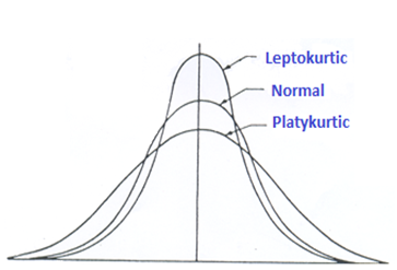
The kurtosis is the standardized fourth central moment. The kurtosis depicts how a random variable is spread out, and unlike the second central moment, it puts more weight on the extreme points.
The kurtosis \(K\) of a random variable \(X\) can be defined as follows:
$$ K=\frac { E\left[ { \left( X-\mu \right) }^{ 4 } \right] }{ { \sigma }^{ 4 } } $$
Two random variables are easily compared by standardizing the central moment. The kurtosis is also similar to skewness in the sense that it will not change even after being multiplied by a constant. The concept of the kurtosis is applicable in finance in the sense that the distribution with a higher kurtosis has a tendency of having more extreme points and is therefore considered riskier, assuming that we have two assets whose distribution of returns are provided, with the same mean, variance, and skewness but with different kurtosis.
The following is the equation of the population kurtosis of a random variable \(X\):
$$ \hat { K } =\frac { 1 }{ n } \sum _{ i=1 }^{ n }{ { \left( \frac { { x }_{ i }-\mu }{ \sigma } \right) }^{ 4 } } $$
The following equation represents the sample statistics kurtosis of a random variable \(X\):
$$ \hat { K } =\frac { n\left( n+1 \right) }{ \left( n-1 \right) \left( n-2 \right) \left( n-3 \right) } \sum _{ i=1 }^{ n }{ { \left( \frac { { x }_{ i }-\hat { \mu } }{ \hat { \sigma } } \right) }^{ 4 } } $$
The normal distribution has a kurtosis of 3. Excess kurtosis is the preferred statistical tool. It is computed as:
$$ { K }_{ excess }=K-3 $$
Supposing that we are to estimate the mean and the variance as well. If we are provided with \(n\) points, then the formula for excess kurtosis becomes:
$$ { \bar { K } }_{ excess }=\bar { K } -3\frac { { \left( n-1 \right) }^{ 2 } }{ \left( n-2 \right) \left( n-3 \right) } $$
\(\bar { K }\) is the sample kurtosis.
The idea of covariance can also be generalized to cross the central moments. The third and fourth standardized cross-central moments are the coskewness and cokurtosis, respectively. Assuming we have \(n\) random variables, then we have the following number of non-trivial order \(m\) moments:
$$ K=\frac { \left( m+n-1 \right) ! }{ m!\left( n-1 \right) ! } -n $$
In non-trivial cross central moments, the cross moments involving only one variable are excluded. The above equation simplifies is simplified to the following form when dealing with coskewness:
$$ { K }_{ 3 }=\frac { \left( n+2 \right) \left( n+1 \right) n }{ 6 } $$
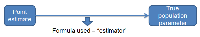
According to tacticians, the best estimator among all the unbiased estimators is one whose variance is the minimum. The estimates produced by this formula are consistently close to the true value of the parameter. Limiting oneself to estimators that are a linear combination of the data, it can be proved that the variance of a given player is the minimum among all the potential unbiased estimators. The estimate possessing all these properties is called the Best Linear Estimator (BLUE).
The probability distribution of the return earned by a newly established hedge fund is as follows:
|
Probability |
Return(%) |
|
20% |
8 |
|
40% |
15 |
|
30% |
20 |
|
10% |
30 |
Calculate the standard deviation of return.
The correct answer is B.
Var(R) = E(R2) – μ2= E(R2) – [E(R)]2
E(R) = 0.2×8 + 0.4×15 + 0.3×20 + 0.1×30 = 16.6
E(R2) = 0.2×82 + 0.4×152 + 0.3×202 + 0.1×302 = 312.8
Var(R) = 312.8 – 16.62 = 37.24
Standard deviation of return = 37.240.5 = 6.1%
From the information given in the table, calculate the portfolio standard deviation.
| Asset 1 | Asset 2 | |
| Weights | 80% | 20% |
| Expected return | 9.98% | 15.80% |
| Standard deviation | 17.00% | 30.00% |
| Cov | 0.005 |
The correct answer is D.
Portfolio return = weighted return of assets
E(Rp) = (0.8 × 9.98%) + (0.2 × 15.8%) = 11.14%
Portfolio variance (σp2) = w12σ12 + w22σ22 + 2w1 w2 ρ12 σ1 σ2
= 0.82 × 0.172 + 0.22 × 0.32 + 2 × 0.8 × 0.2 × 0.005 = 0.023696
Portfolio risk = Portfolio standard deviation = √0.023696 = 0.1539 = 15.39%
Note: The portfolio risk is less than the risk of each respective asset.
Offered by AnalystPrep


