Financial Correlation Modeling – Bottom-Up Approaches

After completing this reading, you should be able to:

• Explain the purpose of copula functions and the translation of the copula equation.
• Describe the Gaussian copula and explain how to use it to derive the joint probability of default of two assets.
• Summarize the process of finding the default time of an asset correlated to all other assets in a portfolio using the Gaussian copula.

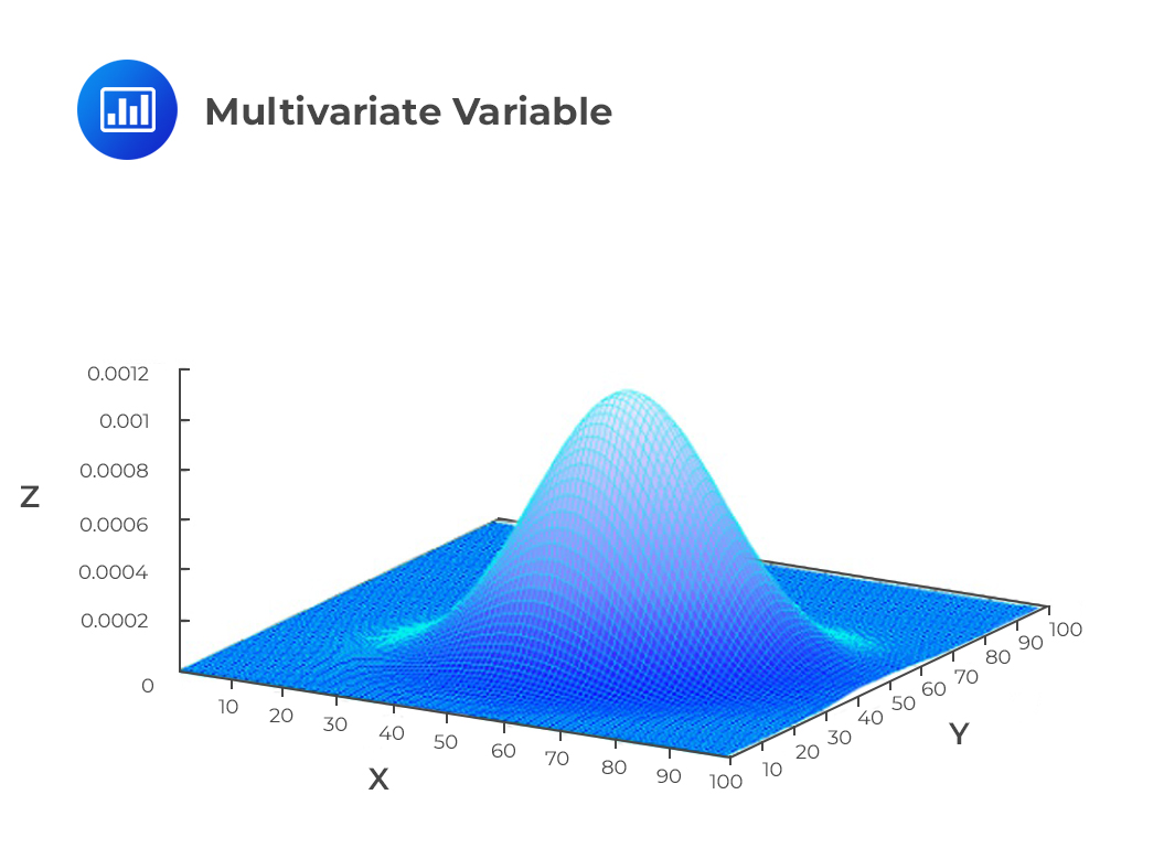
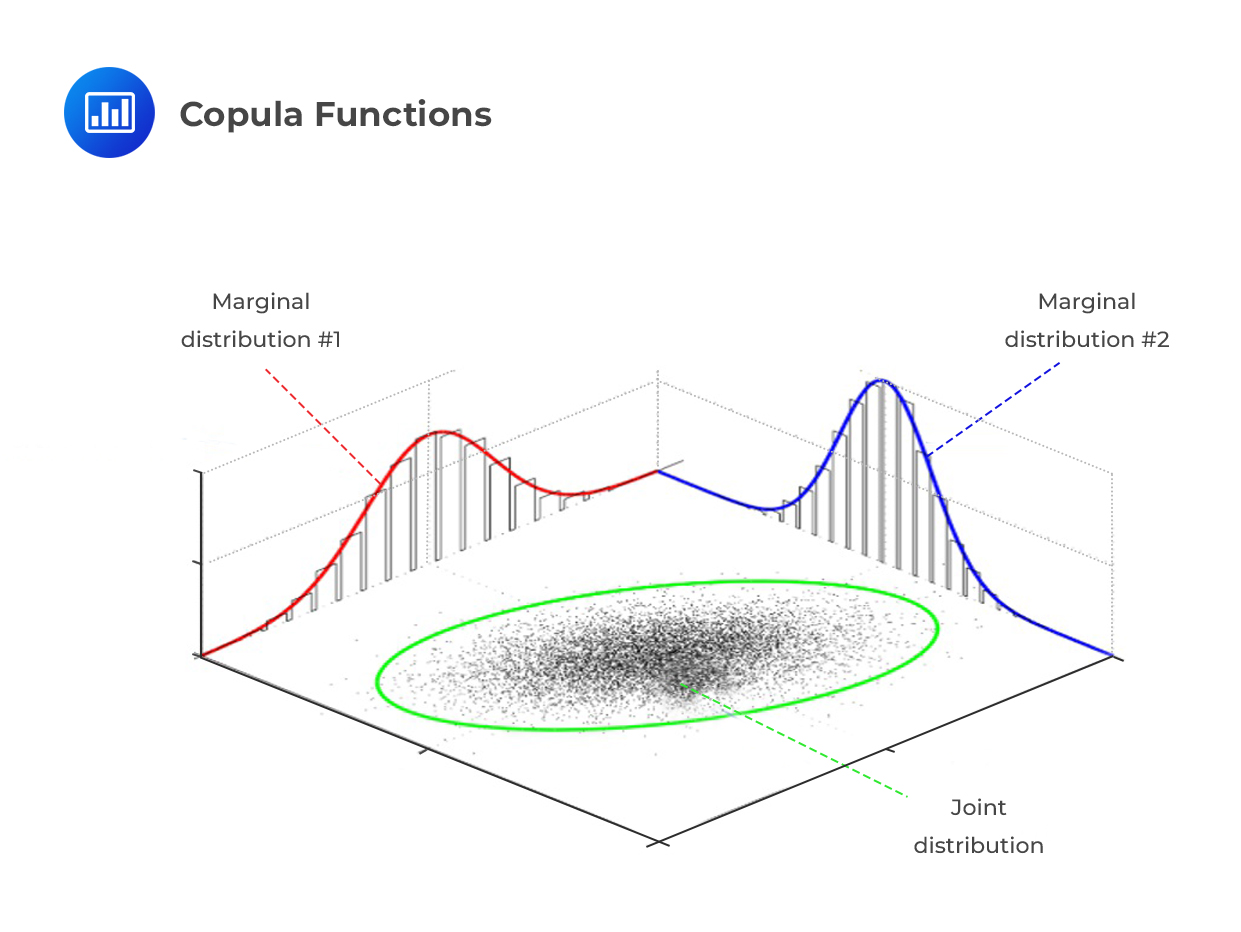
A copula is a multivariate distribution that examines the association or dependence between many variables. They allow the amalgamation of multiple univariate distributions into a single multivariate distribution.

Copulas provide risk managers and market analysts with a measure of the dependence between various financial variables that are not subject to the same limitations as correlation. The correlation only works well with a normal distribution. Nevertheless, as we have established before, financial markets don’t always exhibit properties of a normal distribution. The most important objective of this chapter is to understand how a correlation copula can be created by mapping at least two unknown distributions to a known distribution, such as the normal distribution, whose properties are well known.

Copula Functions

To create a correlation copula, two or more unknown distributions are mapped to a well-known distribution, such as the normal distribution, whose properties are well established. As a result, a joint probability distribution is created while still maintaining the individual (constituent) marginal distributions.

A copula function C transforms an n-dimensional function on the interval [0, 1] into a unit-dimensional one:

$$ \text C: [0, 1]^{\text n} \rightarrow [0, 1] $$

In general, suppose \(\text G_\text i (\text u_\text i) \in [0,1]\) is a univariate, uniform distribution with \(\text u_\text i=\text u_1,…\text u_\text n\) and \(\text i \in \text N\) (i is an element of set N). We, therefore, define a copula function as follows:

$$ \text C[\text G_1 (\text u_1),…,\text G_\text n (\text u_\text n)]=\text F_\text n [\text F_1^{-1} (\text G_1 (\text u_1)),…,\text F_\text n^{-1} (\text G_\text n (\text u_\text n));\rho_\text F ] $$

where:

\(\text G_\text i (\text u_\text i)\) are the marginal distributions that have no well-known properties.

\(\text F_\text n\) is the joint cumulative distribution function.

\(\text F_\text i^{-1}\) is the inverse of \(\text F_\text i\).

\(\rho_\text F\) is the correlation structure of \(\text F_\text n\).

Put in words, the above equation reads:

Given the marginal distributions \(\text G_1 (\text u_1)\) to \(\text G_\text n (\text u_\text n)\), there exists a copula function that allows the mapping of the marginal distributions \(\text G_1 (\text u_1)\) to \(\text G_\text n (\text u_\text n)\) via \(\text F^{-1}\) and the joining of the (abscise values) \(\text F_\text i^{-1} (\text G_\text i (\text u_\text i))\) to a single, n-variate function \(\text F_\text n [\text F_1^{-1} (\text G_1 (\text u_1)),…,\text F_\text n^{-1} (\text G_\text n (\text u_\text n))]\) that has a correlation structure of \(\rho_\text F\).

In essence, therefore, the equation above defines the process where unknown marginal distributions are mapped to a well-known distribution, such as the standard multivariate normal distribution.

Sklar’s Theorem

A key part of copulas is Sklar’s theorem. The theorem states that any multivariate joint distribution can be written in terms of univariate marginal distribution functions and a copula which describes the dependence structure between the variables. Mathematically, the theorem can be stated as follows:

Assume that we have only two random variables, X and Y. If F(x,y) is a joint distribution function with continuous marginals \(\text F_\text x (\text x) = \text u\) and \(\text F_\text y (\text y) =\text v\), then the joint distribution F(x,y) can be written in terms of a unique function C(u,v):

$$ \text F(\text x,\text y)=\text C(\text u,\text v) $$

where C(u,v) is known as the copula of F(x,y).

The copula function describes how the multivariate function F(x,y) is derived from or coupled with the marginal distribution functions \(\text F_\text x(\text x)\) and \(\text F_\text y(\text y)\).

Bottom Line

A copula is a function that ‘joins together’ a collection of marginal distributions to form a multivariate distribution. It can also be interpreted as a representation of the dependence structure of X and Y.

Types of Copulas Functions

There are numerous types of copulas but there are two main classes: one-factor copulas and two-factor copulas.

The most popular one–factor copulas are the Gaussian copula and the Archimedean copula family. The latter can be split further into Gumbel, Clayton, and Frank copulas.

Two-factor copulas include the student’s t copula, Frechet copula, and Marshal-Olkin copula. We concentrate on the Gaussian copula.

Gaussian Copula

A Gaussian copula maps the marginal distribution of each variable to the standard normal distribution which, by definition, has a mean of zero and a standard deviation of one. Copula correlation models create a joint probability distribution for two or more variables while still preserving their marginal distributions. The joint probability of the variables of interest is implicitly defined by mapping them to other variables whose distribution properties are known.

We can demonstrate how Gaussian copulas work using a simple example.

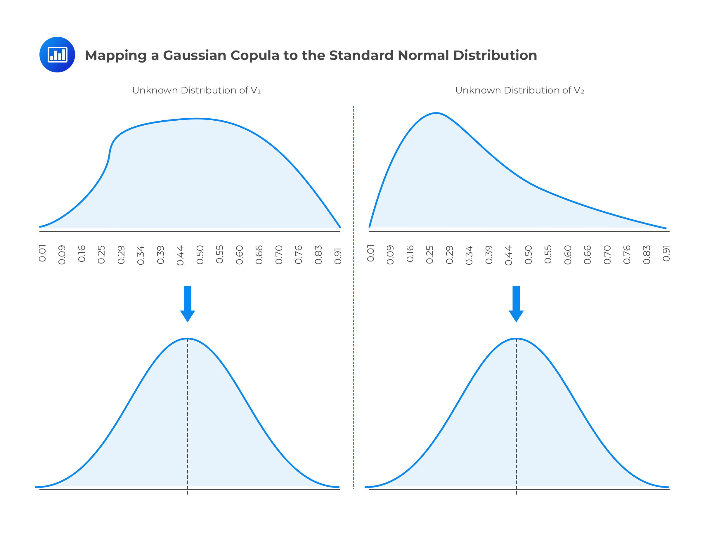
Let’s define two variables \(\text V_1\) and \(\text V_2\) that have unknown distributions and unique marginal distributions. \(\text V_1\) and \(\text V_2\) are mapped into new variables \(\text U_1\) and \(\text U_2\) that have standard normal distributions. The mapping is done on a percentile-to-percentile basis to create a Gaussian copula.

For example, the one-percentile point of the \(\text V_1\) distribution is mapped to the one-percentile point of the \(\text U_1\) distribution. Similarly, the 50-percentile point of the \(\text V_1\) distribution is mapped to the 50-percentile point of the \(\text U_1\) distribution.

Before mapping variables \(\text V_1\) and \(\text V_2\) to the normal distribution, it is very difficult to define the relationship between them since their marginal distributions are unknown and are pretty much incomprehensible structures. Once they have been mapped to the standard normal distribution as new variables \(\text U_1\) and \(\text U_2\), respectively, we can define the relationship between them since the standard normal distribution has a known structure. The Gaussian copula, therefore, helps us to define the correlation between variables when it is not possible to directly define the correlation.

For a total of n variables, the Gaussian copula, \(\text C_\text G\), is defined as follows:

$$ \text C_\text G [\text G_1 (\text u_1 ),…,\text G_\text n (\text u_\text n )]=\text M_\text n [\text N_1^{-1} (\text G_1 (\text u_1 )),…,\text N_\text n^{-1} (\text G_\text n (\text u_\text n ));\rho_\text M ] $$ where:

\(\text M_\text n\) is joint standard multivariate normal distribution.

\(\text N^{-1}\) is the inverse of the univariate standard normal distribution.

\(\rho_\text M\) denotes the n x n correlation matrix for the joint standard multivariate normal distribution \(\text M_\text n\).

If the \(\text G_\text x (\text u_\text x)\) are uniform, then the \(\text N^1 (\text G_\text x (\text u_\text x))\) are standard normal and \(\text M_\text n\) is standard multivariate normal.

Gaussian Copula and Default Risk

We can use the Gaussian default time copula to measure default risk:

$$ \text C_{\text {GD}} [\text Q_1 (\text t),…,\text Q_\text n (\text t)]=\text M_\text n [\text N_1^{-1} (\text Q_1 (\text t)),…,\text N_\text n^{-1} (\text Q_\text n (\text t));\rho_\text M ] $$

This equation reads:

Given marginal distributions of cumulative default probabilities \(\text Q_\text i (\text t)\) of entities i = to n at times t, there exists a Gaussian copula function \(\text C_{\text {GD}}\) which allows the mapping of the marginal distributions \(\text Q_\text i (\text t)\) via \(\text N^{-1}\) to standard normal. Besides, the function allows the joining of the (abscise values) \(\text N_\text n^{-1} (\text Q_\text n (\text t))\) to a single n-variate standard normal distribution \(\text M_\text N\), with the correlation structure \(\rho_\text M\).

The term \(\text N_\text n^{-1} (\text Q_\text n (\text t))\) maps each individual cumulative default probability for asset i for time period t on a percentile-to-percentile basis to the standard normal distribution.

Example: Applying the Gaussian Copula

Assume that a risk manager owns two non-investment grade bonds – rated BB+ and BB. The bonds have been issued by two companies and their default probabilities are as listed below:

$$ \textbf{Default Probabilities for Non-investment Grade Bonds} $$

$$ \begin{array}{c|c|c} \textbf{Time,t} & \textbf{Default probability} & \textbf{Default probability} \\ {} & \bf{\text{Asset} 1 – \text{Rated BB}+} & \bf{\text{Asset} 2 – \text{Rated BB}} \\ \hline {1} & {0.065} & {0.238} \\ \hline {2} & {0.081} & {0.152} \\ \hline {3} & {0.072} & {0.113} \\ \hline {4} & {0.064} & {0.092} \\ \hline {5} & {0.059} & {0.072} \\ \end{array} $$

How can a Gaussian copula be constructed to estimate the joint default probability, Q, of these two companies in the next year, assuming a one-year Gaussian default correlation of 0.4?

Solution

Since we have just two companies, a bivariate standard normal distribution, \(\text M_2\), with a default correlation coefficient of \(\rho\) can be applied. What’s more, only a single correlation coefficient is required, and not a correlation matrix \(\rho_\text M\).

$$ \text C_{\text {GD}} [\text Q_{\text {BB}+} (\text t),\text Q_{\text {BB}} (\text t)]=\text M_2 [\text N_1^{-1} (\text Q_{\text {BB}+} (\text t)),\text N_\text n^{-1} (\text Q_{\text {BB}} (t\text ));\rho_\text M ] $$

First, we have to determine the cumulative probabilities of each asset. We should then map each individual cumulative default probability for each asset for time period t on a percentile-to-percentile basis to the standard normal distribution.

$$ \textbf{Mapping Cumulative Default Probabilities to Standard Normal Distribution} $$

$$ \begin{array}{c|c|c} \textbf{Time, t} & \textbf{Default} & \textbf{Cum.} & \bf{\text N^{-1} (\text Q_{\text{BB}+} (\text t))} & \textbf{Default} & \textbf{Cum.} & \bf {\text N^{-1} (\text Q_{\text{BB}} (\text t))} \\ {} & \textbf{probability} & \textbf{Prob.} & {} & \textbf{probability} & \textbf{Prob.} & {} \\ {} & \textbf{Asset 1 –} & \bf{\text Q_{\text{BB}+} (\text t)} & {} & \bf{\text{Asset} 2 –} & \bf{\text Q_{\text{BB}} (\text t)} & {} \\ {} & \bf{\text{ Rated BB}+} & {} & {} & \textbf{Rated BB} & {} & {} \\ \hline {1} & {0.065} & {0.065} & {-1.5141} & {0.238} & {0.238} & {-0.7123} \\ \hline {2} & {0.081} & {0.146} & {-1.0537} & {0.152} & {0.390} & {-0.2793} \\ \hline {3} & {0.072} & {0.218} & {-0.7790} & {0.113} & {0.503} & {0.0075} \\ \hline {4} & {0.064} & {0.282} & {-0.5769} & {0.092} & {0.595} & {0.2404} \\ \hline {5} & {0.059} & {0.341} & {-0.4097} & {0.072} & {0.667} & {0.4316} \\ \end{array} $$

We map the cumulative default probabilities Q(t) to the standard normal distribution via \(\text N^{−1}(\text Q(\text t))\). Although it is possible to do this manually, the computation is easier and much faster when using the Excel Function =NORM.S.INV(Q(t)) or the MATLAB® function =NORMINV(Q(t)).

The copula model assumes that we can apply the correlation structure \(\rho_\text M\) or a single ρ of the multivariate distribution (in this case the Gaussian multivariate distribution) to the transformed marginal distributions \(\text N^{-1} (\text Q_{\text {BB}+} (\text t))\) and \(\text N^{-1} (\text Q_{\text {BB}} (\text t))\).

The joint probability of both Company B and Company C defaulting within one year is calculated as:

$$ \text Q(\text t_{\text {BB}+} \le 1\cap \text t_{\text {BB}} \le 1)\equiv \text M(\text X_{\text {BB}+}\le -1.5141 \cap \text X_{\text {BB}} \le -0.7123,\rho=0.4)=3.4\% $$

where \(\text t_{\text {BB}+}\) is the default time of the issuer of asset 1 and \(\text t_{\text {BB}}\) is the default time of the issuer of asset 2. \(\text X_{\text {BB}+}\) and \(\text X_{\text {BB}}\) are the mapped abscise values of the bivariate normal distribution, derived from the table above.

Exam Note: Calculating percentiles for mapping on to the standard normal distribution is computationally intensive and you are unlikely to be asked to do it on exam day. You are also unlikely to be asked to compute the joint probability of default. The important thing here is to grasp how to go about the process.

Default Time of an Asset Correlated to All Other Assets in a Portfolio Using the Gaussian Copula

The Gaussian copula can also be used to derive the default time relationships when there are more than two random variables (assets) in a portfolio. A Cholesky decomposition is used to derive a sample \(\text {Mn} (\bullet )\) from a multivariate copula \(\text {Mn} (\bullet ) \in [0,1]\).

The default correlations of the sample are determined by the default correlation matrix, \(\rho_\text M\), for the n-variate standard normal distribution, \(\text M_\text n\).

First, we equate the sample (\(\bullet\)) from \(\text M_\text n, \text {Mn} (\bullet)\) to the cumulative individual default probability Q of asset i at \(\text{time } \tau, \text Q_\text i (\tau_\text i)\). This can be accomplished using Microsoft Excel® or a Newton-Raphson search procedure. Therefore,

$$ \begin{align*} \text {Mn} (\bullet) & =\text Q_\text i (\tau_\text i) \\ \text{Or } \tau_\text i & =\text Q_\text i^{-1} (\text {Mn} (\bullet)) \\ \end{align*} $$

Example: Estimating Default Time

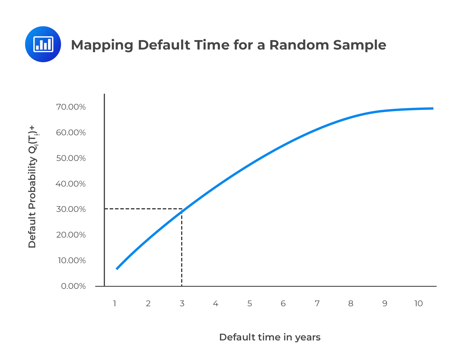
Assume that we have drawn a 30% cumulative default probability for asset i from a random n-variate standard normal distribution, \(\text {Mn} (\bullet)\).

The n-variate standard normal distribution includes a default correlation matrix, \(\rho_\text M\), that gives all of the assets’ default correlations with all n assets. The figure below illustrates how to equate this 30% with the market-determined cumulative individual default probability, \(\text Q_\text i (\tau_\text i)\). We note that 30% coincides with \(\tau=3\). To find our estimate of default time \(\tau_\text i\), we repeat this procedure numerous times, for example, 100,000 times, and average each \(\tau_\text i\) of every simulation.

Applications of Copula Functions in Finance

Copulas are used to model risk in collateralized debt obligations (CDOs).

CDOs are divided into tranches where each tranche represents a group of investors with different risk degrees. The CDO’s overall risk is distributed over all the tranches. To determine the price of a given tranche of a CDO, risk managers will need the following: the default probability, the default severity (or recovery), and the default correlation. The default correlation represents the likelihood that the default of one asset causes the default of another. Note that default correlation is much higher between credits within the same industrial sector. Default correlations can be modeled through the use of the one-factor copula model.

Copulas are also popular tools to model credit default swaps with counterparty risk. In most cases, risk managers apply the bivariate Gaussian copula to model the default correlation between the CDS seller and the reference asset.

In recent years, copulas have also emerged as useful tools in the modeling of constant maturity spread options, foreign exchange cross options, and basket options.

Drawbacks of Gaussian Copula

The Gaussian copula approach, unfortunately, cannot model tail dependence. This implies that the use of the Gaussian copula to model risk in CDOs results in an underestimation of extreme events in the upper and lower tails of the joint distribution of several random variables. In particular, the approach does not consider the simultaneous default of a large number of assets in the underlying portfolio. The inability of the Gaussian copula to model tail dependence has shared part of the blame for the 2007/2009 financial crisis.

Question

Which of the following correctly describes the purpose of copula functions and their application in finance?

A. Copula functions are used to evaluate linear relationships between assets and are best suited for portfolios with straightforward correlation structures.

B. Copula functions provide a measure of how the return on one asset impacts the volatility of another asset in the portfolio.

C. Copula functions allow for modeling dependencies between assets by separating marginal distributions from their copula, providing a more flexible approach to understanding complex correlation structures.

D. Copula functions primarily assess the tail risks associated with individual assets, without considering the dependencies between them.

Solution

The correct answer is C.

Copula functions are a mathematical tool that allows for the modeling of dependencies between random variables. In finance, this is particularly useful for understanding the correlation structures between different assets. The primary advantage of copula functions is that they separate the marginal distributions of individual assets from their copula, allowing for a more flexible and detailed analysis of dependencies, especially when relationships are non-linear or more intricate.

A is incorrect because copula functions are not just used to evaluate linear relationships. In fact, their main strength lies in analyzing non-linear dependencies and more complex correlation structures, which standard correlation measures might not capture adequately.

B is incorrect because copula functions do not focus on how the return of one asset impacts the volatility of another. Instead, they analyze the dependency structure between multiple assets.

D is incorrect because copulas are specifically designed to analyze the dependencies between variables. While they can be used in the context of assessing tail dependencies, they do not exclusively focus on individual asset tail risks without considering inter-asset dependencies.

Things to Remember

• Copula functions are mathematical tools utilized to model the dependencies between random variables.
• In finance, copulas help in analyzing the correlation structures between various assets, especially in contexts where relationships might be non-linear or intricate.
• One key strength of copula functions is the separation of marginal distributions of individual assets from their joint dependency structure. This separation facilitates a more nuanced understanding of asset dependencies.
• Copulas offer flexibility in modeling complex correlation structures that standard correlation measures might not capture comprehensively.
• The primary focus of copula functions is not on individual asset risks but on the interdependencies between them.